👀 FAQ#
Need some help to setup python for EOmaps?#
Have a look at the Quickstart Guide to learn how to setup a python environment that can be used to create EOmaps maps!
Interested in contributing to EOmaps?#
Have a look at the Contribution Guide on how to setup a development environment to start contributing to EOmaps! Any contributions are welcome!
Configuring the editor (IDE)#
EOmaps can be used with whatever editor you like!
However, for some editors there are special settings that can be adjusted to improve your mapping experience with EOmaps:
Spyder
To use the whole potential of EOmaps with the awesome Spyder IDE ,
the plot-settings must be adjusted to ensure that matplotlib plots are created as interactive Qt widgets.
By default, figures are rendered as static images into the plots-pane. To avoid this and create interactive (popup) figures instead, go to the preferences and set the “Graphics Backend” to “Automatic” :
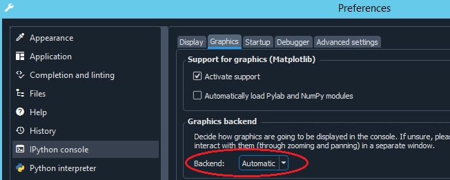
Note
If the gaphics-backend is set to “Automatic”, you can still plot static snapshots of a figure to the “plots-pane” with Maps.snapshot()!
VSCode / VSCodium
In general, EOmaps should work “out of the box” with VSCode or the open-source variant VSCodium (together with the standard Python extension).
However, there are some tipps that might help with your mapping workflow:
In a normal python-terminal, the default matplotlib backend will be
QtAggin a non-interactive mode. This means that you must callMaps.show()at the end of the script to actually show the figure. Once the figure is shown, the terminal is blocked until the figure is closed.To avoid blocking the terminal while a figure is running, you can activate matplotlib’s interactive-mode using
from eomaps import Maps
Maps.config(use_interactive_mode=True)
Once activated, figures are immediately shown as soon as a new
Mapsobject is created and the terminal is not blocked (e.g. you can continue to execute commands that update the figure).
Note
If you run a whole script using the interactive mode, the script will run until the end and then usually terminate the associated kernel… and in turn also closing the figure! If you want to keep the figure open, either make sure that the terminal is kept alive by entering debug-mode, or avoid activating the interactive mode and block the terminal with m.show().
If you enjoy interactive coding in a Jupyter-Notebook style, make sure to have a look at the nice Jupyter extension!
It allows you to work with an interactive IPython terminal and execute code-blocks (separated by the # %% indicator).
With IPython, the default behavior is to create static (inline) figures (same as with Jupyter Notebooks)!
To print a snapshot of the current state of a figure to the IPython terminal, call
Maps.show()orMaps.snapshot().Similar to Jupyter Notebooks, you can use “magic” commands to set the used matplotlib backend.
For interactive (popup) figures, switch to the default Qt backend using
%matplotlib qtFor interactive (inline) figures, you’ll need to install ipympl and then activate the
widgetwith%matplotlib widget.For more details, see details on Jupyter Notebooks below!
PyCharm
The PyCharm IDE automatically registers its own matplotlib backend which (for some unknown reason) freezes on interactive plots.
To my knowledge there are 2 possibilities to force pycharm to use the original matplotlib backends:
- 🚲 The “manual” way:Add the following lines to the start of each script:(for more info and alternative backends see matplotlib docs)
import matplotlib
matplotlib.use("Qt5Agg")
- 🚗 The “automatic” way:Go to the preferences and add the aforementioned lines to the “Starting script”(to ensure that the
matplotlibbackend is always set prior to running a script)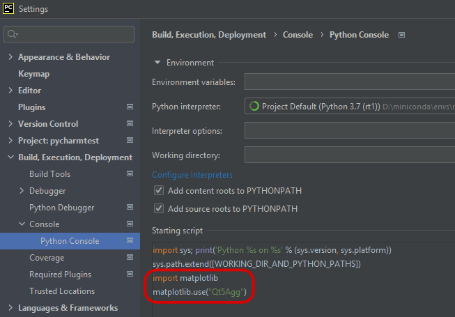
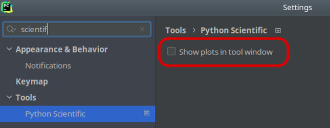
In addition, if you use a commercial version of PyCharm, make sure to disable “Show plots in tool window” in the Python Scientific preferences since it forces plots to be rendered as static images.
Jupyter Notebooks
When working with Jupyter Notebooks, we recommend to use Jupyter Lab.
By default, EOmaps will use the
inlinebackend and put a static snapshot of the current state of the figure to the Jupyter Notebook cell whenever you callMaps.show()orMaps.snapshot().To get interactive inline figures in Jupyter Notebooks, you have to switch to the ipympl (
widget) backend.To install, use
conda install -c conda-forge ipymplOnce it’s installed, you can use the “magic command”
%matplotlib widgetat the start of the code to activate the backend.
To use the 🧰 Companion Widget in backends other than Qt the Qt event-loop must be integrated.
This can be done with the %gui qt command.
%matplotlib widget
%gui qt

from eomaps import Maps
m = Maps()
m.add_feature.preset("coastline", "ocean")
For classical notebooks, there’s also the
nbaggbackend provided by matplotlibTo use it, simply execute the magic
%matplotlib notebookbefore starting to plot.
You can also use the magic
%matplotlib qtto use the defaultqt5aggbackend.This way the plots will NOT be embedded in the notebook, they show up as interactive popup figures!
Note
Irrespective of the used backend, you can always plot a static snapshots of the current state of a map to a Jupyter Notebook
with Maps.snapshot()!
%matplotlib qt    # Create figures as interactive popup widgets

from eomaps import Maps
m = Maps()
m.add_feature.preset("coastline", "ocean")
m.snapshot()      # Print a snapshot of the current state of the figure to the Jupyter Notebook
Checkout the matplotlib doc for more info!
Record interactive maps to create animations#
The best way to record interactions on a EOmaps map is with the free and open source ScreenToGif software.
All animated gifs in this documentation have been created with this awesome piece of software.
LICENSING and redistribution#
Information is provided WITHOUT WARRANTY FOR CORRECTNESS!
Since v8.0, the source-code of EOmaps is licensed under a BSD 3-clause license.
However, it must be notet that EOmaps has a number of required and optional dependencies whose licenses must be taken into account when packaging and redistributing works that build on top of EOmaps. While most dependencies are either BSD or MIT licensed, there are some dependencies that might require additional considerations.
Most notably (start of 2024), the required dependency cartopy is licensed under LGPLv3+ (however they are in the process of re-licensing to BSD-3-clause) and the optional Qt GUI framework is available via commertial and open-source (LGPLv3+) licenses and the used python-bindings (PyQt5) are licensed under GPL v3.
Tip
If you want to get a quick overview of the licenses of an existing python environment, I recommend having a look at the pip-licenses package!
Important changes between major versions#
⚙ From EOmaps v3.x to v4.x
Changes between EOmaps v3.x and EOmaps v4.0:
the following properties and functions have been removed:
❌
m.plot_specs.❌
m.set_plot_specs()- arguments are now directly passed to relevant functions:
m.plot_map(),m.add_colorbar()andm.set_data()
🔶
m.set_shape.voroni_diagram()is renamed tom.set_shape.voronoi_diagram()- 🔷 custom callbacks are no longer bound to the Maps-objectthe call-signature of custom callbacks has changed to:
def cb(self, *args, **kwargs)>>def cb(*args, **kwargs)
Porting a script from v3.x to v4.x is quick and easy and involves the following steps:
Search your script for all occurrences of the words
.plot_specsand.set_plot_specs(, move the affected arguments to the correct functions (and remove the calls once you’re done):vmin,vmaxalphaandcmapare now set inm.plot_map(vmin=..., vmax=..., alpha=..., cmap=...)histbins,label,tick_precisionanddensityare now set inm.add_colorbar(histbins=..., label=..., tick_precision=..., density=...)cposandcpos_radiusare now (optionally) set inm.set_data(data, x, y, cpos=..., cpos_radius=...)
Search your script for all occurrences of the words
xcoordandycoordand replace them withxandyONLY if you used voronoi diagrams:
search in your script for all occurrences of the word
voroni_diagramand replace it withvoronoi_diagram
ONLY if you used custom callback functions:
the first argument of custom callbacks is no longer identified as the
Mapsobject.if you really need access to the
Mapsobject within the callback, pass it as an explicit argument!
EOmaps v3.x:
m = Maps()
m.set_data(data=..., xcoord=..., ycoord=...)
m.set_plot_specs(vmin=1, vmax=20, cmap="viridis", histbins=100, cpos="ul", cpos_radius=1)
m.set_shape.voroni_diagram()
m.add_colorbar()
m.plot_map()

# ---------------------------- custom callback signature:
def custom_cb(m, asdf=1):
    print(asdf)

m.cb.click.attach(custom_cb)
EOmaps v4.x:
m = Maps()
m.set_data(data=..., x=..., y=..., cpos="ul", cpos_radius=1)
m.plot_map(vmin=1, vmax=20, cmap="viridis")
m.set_shape.voronoi_diagram()
m.add_colorbar(histbins=100)

# ---------------------------- custom callback signature:
def custom_cb(**kwargs, asdf=None):
    print(asdf)

m.cb.click.attach(custom_cb, asdf=1)
Note: if you really need access to the maps-object within custom callbacks, simply provide it as an explicit argument!
def custom_cb(**kwargs, m=None, asdf=None):
    ...

m.cb.click.attach(custom_cb, m=m, asdf=1)
⚙ From EOmaps v5.x to v6.x
General changes in behavior
- 🔶 Starting with EOmaps v6.0 multiple calls to
m.plot_map()on the same Maps-object completely remove (and replace) the previous dataset!(use a new Maps-object on the same layer for datasets that should be visible at the same time!) - 🔶 WebMap services are no longer re-fetched by default when exporting images with
m.savefig()To force a re-fetch of WebMap services prior to saving the image at the desired dpi, usem.savefig(refetch_wms=True)(seem.refetch_wms_on_size_change()for more details) - 🔷
m.add_gdfnow uses only valid geometries(to revert to the old behavior, use:m.add_gdf(..., only_valid=False)) 🔷 the order at which multi-layers are combined now determines the stacking of the artists
m.show_layer("A|B")plots all artists of the layer"A"on top of the layer"B"the ordering of artists inside a layer is determined by their
zorder(e.g.m.plot_map(zorder=123))
Removed (previously depreciated) functionalities
❌ the
m.figureaccessor has been removed!Use
m.ax,m.f,m.colorbar.ax_cb,m.colorbar.ax_cb_plotinstead
❌ kwargs for
m.plot_map(...)"coastlines"usem.add_feature.preset.coastline()instead
❌ kwargs for
m.set_data(...)"in_crs"use"crs"instead"xcoord"use"x"instead"ycoord"use"y"instead
❌ kwargs for
Maps(...)"parent"… no longer needed"gs_ax"use"ax"instead
❌ kwargs for
m.new_inset_maps(...)"edgecolor"and"facecolor"useboundary=dict(ec=..., fc=...)instead
❌ kwargs for
m.add_colorbar(...)"histbins"use"hist_bins"instead"histogram_size"use"hist_size"instead"density"use"hist_kwargs=dict(density=...)"instead"top", "bottom", "left", "right"usemargin=dict(top=..., bottom=..., left=..., right=...)instead"add_extend_arrows"
❌
m.indicate_masked_points()has been removed, usem.plot_map(indicate_masked_points=True)instead❌
m.shape.get_transformeris now a private (e.g.m.shape._get_transformer)❌
m.shape.radius_estimation_rangeis now a private (e.g.m.shape._radius_estimation_range)
⚙ From EOmaps v6.x to v7.x
⚠️ A lot of internal functions and classes have been re-named to better follow PEP8 naming conventions. While this should not interfere with the public API, more extensive customizations might need to be adjusted with respect to the new names.
If you encounter any problems, feel free to open an issue , and I’ll see what I can do!
For example: the module _shapes.py is now called shapes.py and the class shapes is now called Shapes
⚠️ The use of
m.set_data_specs(...)is depreciated. Usem.set_data(...)instead!Figure export routines have been completely re-worked (but should result in the exact same output as in v6.x)
⚙ From EOmaps v7.x to v8.x
❗ Starting with v8.x eomaps is licensed under a “BSD 3 clause” license!
⚠️ Some functions and classes have been re-named/moved to better follow PEP8 naming conventions. While this should not interfere with the public API, more extensive customizations might need to be adjusted with respect to the new names.
If you encounter any problems, feel free to open an issue , and I’ll see what I can do!
⚠️
pipinstall has been updated to implement optional dependency groups.❗
pip install eomapsnow only installs minimal dependencies required for eomapsHave a look at the 🐛 Installation instructions for more details!
setup.pyand_version.pyhave been removed in favor of using apyproject.tomlfilescripts for the examples have been re-named and are now located in
docs\examplesColorbar kwargs
show_outlineandylabelhave been renamed tooutlineandhist_label
The following (previously deprecated) methods are now removed:
m.set_data_specs -> use
m.set_datainsteadm.add_wms.DLR_basemaps… -> use
m.add_wms.DLR.basemap...insteadm_inset.indicate_inset_extent -> use
m_inset.add_extent_indicatorinstead
There have been substantial changes to the internals of the callback machinery
The public
MapsAPI is unaffectedChanges are primarily in the modules
cb_container.pyandcallbacks.py