👀 FAQ
🚀 From 0 to EOmaps - a quickstart guide
The following section is intended to provide a quick overview on how to get started using EOmaps.
The guide is intended to be concise and covers only the most important information to get things running. Links to websites that provide additional information are provided throughout the text.
Note
This tutorial is intended to get you up and running from scratch as fast as possible using 100% free and open-source tools. It does not cover alternative ways on how to setup python or how to use alternative editors etc.
Feel free to start a discussion of open an issue if you have additional questions or suggestions!
Prerequisites:
A computer (Windows / MacOS / Linux) - no root access required
basics on how to work with a terminal
basic python knowledge
🐍 Getting started - set up a python environment
There are of course many ways to set up a python environment… in the following, we will use the (free and open-source) conda
package manager which greatly simplifies the creation of environments that depend on both python and c++ libraries
(A lot of python-packages for geo-libraries are just bindings to c++ libraries such as GDAL or PyProj).
conda is available for MacOS, Windows and Linux.
For more details, see conda-docs .
The fastest way to get started is to use miniconda, a minimalistic installer that includes only
conda, python and a minimal set of additional packages.
TODO (~10 min)
Download and install the latest version of miniconda from:
After the installation is finished, open a Anaconda Prompt terminal (if you need help, see “starting conda” ).
By default, the terminal starts in the conda-environment base (you should see the name in brackets on the left).
Before creating a new dedicated python-environment, we’ll first install mamba into the base environment
to speedup the installation process. (for details on mamba, have a look at the mamba-docs !)
NOTE: The use of
mambais optional (but highly recommended)! If you don’t want to use it, just replace the termmambawithcondain all subsequent commands.
TODO (~1 min) install mamba:
Install mamba from the conda-forge channel with the following command (in the Anaconda Prompt terminal):
conda install -c conda-forge mamba
Now that mamba is installed, we can use it to create a new python environment, and install the following packages:
As editor to write and execute python-code we will use the awesome (free and open-source) spyder-IDE
in addition, we install
eomapsandmatplotlib(the latter is only required to make sure matplotlib backends such as Qt5Agg are installed)all required dependencies will be automatically determined and installed during the process
TODO (~15 min, ~500mb) setup environment:
Setup a new python environment named eomaps and install
EOmaps and the spyder IDE.
mamba create -n eomaps -c conda-forge spyder eomaps matplotlib
Once the list of required packages is determined, confirm the installation with y and wait until
it is completed.
Finally, all that’s left to do is to activate the environment and start the editor!
TODO (~1 min) activate environment, start and setup the spyder IDE:
To activate the environment, use:
conda activate eomaps
After activating the environment, we can start the spyder IDE with:
spyder
As a last step, we need to adjust the default plot-settings of the spyder IDE to make sure that
matplotlib plots are generated as interactive widgets
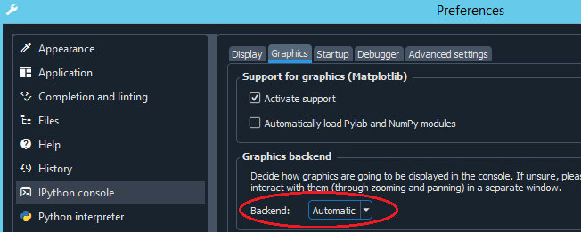
By default, plots are rendered as static images into the “plots-pane”… to avoid this and create interactive
matplotlibwidgets instead, go to the preferences, select the IPython console section and set the Graphics backend to Automatic :
Now you’re ready for your first map! -> head over to 🌐 EOmaps examples and run one of the example-codes!
A few quick spyder IDE tips:
In spyder you will work with an interactive IPython console.
This allows you to dynamically execute parts of a script and immediately see the outcome.
use
F9to execute the selected code (or the current line if nothing is selected)use
F5to execute the current script (e.g. the whole file)use
shift + enterto execute the currently selected code-block (code-blocks are separated by# %%)
💻 Configuring the editor (IDE)
🕷 Spyder IDE
To use the whole potential of EOmaps with the awesome Spyder IDE ,
the plot-settings must be adjusted to ensure that matplotlib plots remain interactive.
By default, plots are rendered as static images into the “plots-pane”… to avoid this and create interactive
matplotlibwidgets instead, go to the preferences and set the “Graphics backend” to “Automatic” :
🗖 PyCharm IDE
The PyCharm IDE automatically registers its own matplotlib backend which (for some unknown reason) freezes on interactive plots.
To my knowledge there are 2 possibilities to force pycharm to use the original matplotlib backends:
- 🚲 The “manual” way:Add the following lines to the start of each script:(for more info and alternative backends see matplotlib docs)
import matplotlib
matplotlib.use("Qt5Agg")
- 🚗 The “automatic” way:Go to the preferences and add the aforementioned lines to the “Starting script”(to ensure that the
matplotlibbackend is always set prior to running a script)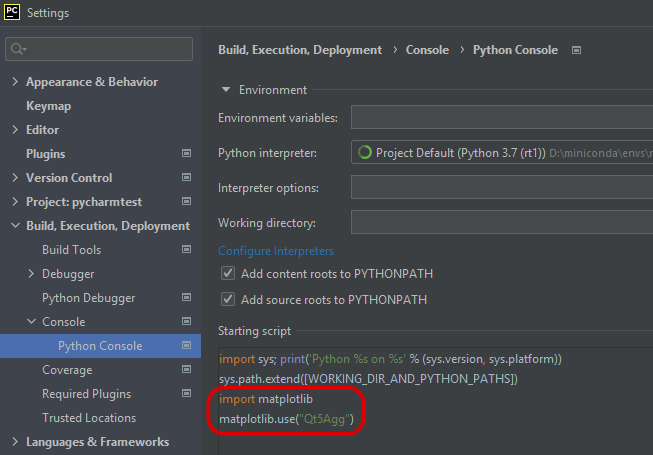
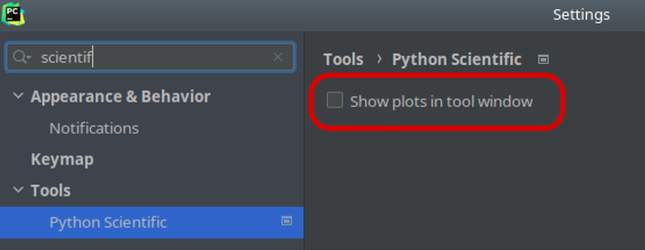
In addition, if you use a commercial version of PyCharm, make sure to disable “Show plots in tool window” in the Python Scientific preferences since it forces plots to be rendered as static images.
📓 Jupyter Notebooks
While EOmaps works best with matplotlib’s Qt5Agg backend, most of the functionalities work
reasonably well if you want the figures embedded in a Jupyter Notebook.
🔸 For jupyter-lab (and classic notebooks) you can use the ipympl backend
To install, simply use
conda install -c conda-forge ipymplOnce it’s installed, (and before you start plotting) use the magic
%matplotlib widgetto activate the backend.See here for more details: https://github.com/matplotlib/ipympl
🔸 For classical notebooks, there’s also the nbagg backend provided by matplotlib
To use it, simply execute the magic
%matplotlib notebookbefore starting to plot.
🔸 Finally, you can also use the magic %matplotlib qt and use the qt5agg backend within Jupyter Notebooks!
This way the plots will NOT be embedded in the notebook but they are created as separate widgets.
Note
It is possible to plot static snapshots of the current state of a map to a Jupyter Notebook irrespective of the used backend by using m.snapshot(), e.g.:
m = Maps()
m.add_feature.preset.coastline()
m.snapshot()
Checkout the matplotlib doc for more info!
📸 Record interactive maps to create animations
The best way to record interactions on a EOmaps map is with the free and open source ScreenToGif software.
All animated gifs in this documentation have been created with this awesome piece of software.
⚙ Port script from EOmaps v3.x to v4.x
Changes between EOmaps v3.x and EOmaps v4.0:
the following properties and functions have been removed:
❌
m.plot_specs.❌
m.set_plot_specs()- arguments are now directly passed to relevant functions:
m.plot_map(),m.add_colorbar()andm.set_data()
🔶
m.set_shape.voroni_diagram()is renamed tom.set_shape.voronoi_diagram()- 🔷 custom callbacks are no longer bound to the Maps-objectthe call-signature of custom callbacks has changed to:
def cb(self, *args, **kwargs)>>def cb(*args, **kwargs)
Porting a script from v3.x to v4.x is quick and easy and involves the following steps:
Search your script for all occurrences of the words
.plot_specsand.set_plot_specs(, move the affected arguments to the correct functions (and remove the calls once you’re done):vmin,vmaxalphaandcmapare now set inm.plot_map(vmin=..., vmax=..., alpha=..., cmap=...)histbins,label,tick_precisionanddensityare now set inm.add_colorbar(histbins=..., label=..., tick_precision=..., density=...)cposandcpos_radiusare now (optionally) set inm.set_data(data, x, y, cpos=..., cpos_radius=...)
Search your script for all occurrences of the words
xcoordandycoordand replace them withxandyONLY if you used voronoi diagrams:
search in your script for all occurrences of the word
voroni_diagramand replace it withvoronoi_diagram
ONLY if you used custom callback functions:
the first argument of custom callbacks is no longer identified as the
Mapsobject.if you really need access to the
Mapsobject within the callback, pass it as an explicit argument!
EOmaps v3.x:
m = Maps()
m.set_data(data=..., xcoord=..., ycoord=...)
m.set_plot_specs(vmin=1, vmax=20, cmap="viridis", histbins=100, cpos="ul", cpos_radius=1)
m.set_shape.voroni_diagram()
m.add_colorbar()
m.plot_map()

# ---------------------------- custom callback signature:
def custom_cb(m, asdf=1):
    print(asdf)

m.cb.click.attach(custom_cb)
EOmaps v4.x:
m = Maps()
m.set_data(data=..., x=..., y=..., cpos="ul", cpos_radius=1)
m.plot_map(vmin=1, vmax=20, cmap="viridis")
m.set_shape.voronoi_diagram()
m.add_colorbar(histbins=100)

# ---------------------------- custom callback signature:
def custom_cb(**kwargs, asdf=None):
    print(asdf)

m.cb.click.attach(custom_cb, asdf=1)
Note: if you really need access to the maps-object within custom callbacks, simply provide it as an explicit argument!
def custom_cb(**kwargs, m=None, asdf=None):
    ...

m.cb.click.attach(custom_cb, m=m, asdf=1)