⚙ Usage

🚀 Basics

🌐 Initialization of Maps objects

EOmaps is all about Maps objects.

To start creating a new map (in this case a plot in epsg=4326, e.g. lon/lat), simply use:

from eomaps import Maps
m = Maps(crs=4326, layer="first layer", figsize=(10, 5))
m.add_feature.preset.coastline()

crs represents the projection used for plotting
layer represents the name of the layer associated with the Maps-object (see below)
all additional keyword arguments are forwarded to the creation of the matplotlib-figure (e.g.: figsize, frameon, edgecolor etc).

Possible ways for specifying the crs for plotting are:

If you provide an integer, it is identified as an epsg-code (e.g. 4326, 3035, etc.)
- 4326 defaults to PlateCarree projection
All other CRS usable for plotting are accessible via Maps.CRS, e.g.: crs=Maps.CRS.Orthographic(), crs=Maps.CRS.GOOGLE_MERCATOR or crs=Maps.CRS.Equi7_EU. (Maps.CRS is just an accessor for cartopy.crs.
- For a full list of available projections see: Cartopy projections)

▤ Layers

A map can have multiple plot-layers.

Each Maps object represents a collection of features on the assigned layer.

Once you have created your first Maps object, you can:

Create additional Maps objects on the same layer by using m2 = m.new_layer()
- If no explicit layer-name is provided, m2 will use the same layer as m
- This is especially useful if you want to plot multiple datasets on the same layer
Create a NEW layer named "my_layer" by using m2 = m.new_layer("my_layer")

Map-features, colorbars and callbacks are layer-sensitive!

Features, colorbars etc. added to a Maps object are only visible if the associated layer is visible
Callbacks are only executed if the associated layer is visible

To switch between layers, use m.show_layer("the layer name"), call m.show() or have a look at the 🦜 Utility widgets and the 🧰 Companion Widget.

m = Maps()                           # same as `m = Maps(layer="base")`
m.add_feature.preset.coastline()     # add some coastlines

m_ocean = m.new_layer(layer="ocean") # create a new layer named "ocean"
m_ocean.add_feature.preset.ocean()   # features on this layer will only be visible if the "ocean" layer is visible!

m2 = m_ocean.new_layer()             # "m2" is just another Maps-object on the same layer as "m_ocean"!
m2.set_data(data=[.14,.25,.38],
            x=[1,2,3], y=[3,5,7],
            crs=4326)
m2.set_shape.ellipses(n=100)
m2.plot_map()

m.show_layer("ocean")                # show the "ocean" layer
m.util.layer_selector()              # get a utility widget to quickly switch between existing layers

The “all” layer

There is one layer-name that has a special meaning… the "all" layer.

Any callbacks and features added to this layer will be executed on ALL other layers as well!

You can add features and callbacks to the all layer via:

using the shortcut m.all. ...
creating a dedicated Maps object via m_all = Maps(layer="all") or m_all = m.new_layer("all")
using the “layer” kwarg of functions e.g. m.plot_map(layer="all")

m = Maps()
m.all.add_feature.preset.coastline() # add some coastlines to ALL layers of the map

m_ocean = m.new_layer(layer="ocean") # create a new layer named "ocean"
m_ocean.add_feature.preset.ocean()
m.show_layer("ocean")                # show the "ocean" layer (note that it has coastlines as well!)

Combining multiple layers

To create a layer that represents a combination of multiple existing layers, separate the individual layer-names

with a "|" character (e.g. "layer1|layer2").

The layer will then always show all features of "layer1 and layer2.

NOTE: The vertical stacking of features is controlled by the zorder property, not by the order of the layers!

m = Maps(layer="first")
m.add_feature.preset.ocean(alpha=0.75, zorder=2)

m2 = m.new_layer("second")                # create a new layer and plot some data
m2.set_data(data=[.14,.25,.38],
            x=[1,2,3], y=[3,5,7],
            crs=4326)
m2.set_shape.ellipses(n=100)
m2.plot_map(zorder=1)                     # plot the data "below" the ocean

m.show_layer("first|second")  # show all features of the two layers

# you can even create Maps-objects representing combined layers!
# (the features will only be visible if all sub-layers are visible)
m_combined = m.new_layer("first|second")
m_combined.add_annotation(xy=(2, 5), xy_crs=4326, text="some text")

`Maps`	The base-class for generating plots with EOmaps.
`Maps.new_layer`	Create a new Maps-object that shares the same plot-axes.
`Maps.all`	Get a Maps-object on the "all" layer.
`Maps.show_layer`	Display the selected layer on the map.
`Maps.show`	Make the layer of this Maps-object visible.
`Maps.fetch_layers`	Fetch (and cache) the layers of a map.

🔵 Setting the data and plot-shape

To assign a dataset to a Maps object, use m.set_data(...).

Maps.set_data

Set the properties of the dataset you want to plot.

A dataset is fully specified by setting the following properties:

data : The data-values
x, y: The coordinates of the provided data
crs: The coordinate-reference-system of the provided coordinates
parameter (optional): The parameter name
encoding (optional): The encoding of the data
cpos, cpos_radius (optional): the pixel offset

The following data-types are accepted as input:

pandas DataFrames `data`: `pandas.DataFrame` `x`, `y`: The column-names to use as coordinates (`string`) `parameter`: The column-name to use as data-values (`string`)	from eomaps import Maps import pandas as pd df = pd.DataFrame(dict(lon=[1,2,3], lat=[2,5,4], data=[12, 43, 2])) m = Maps() m.set_data(df, x="lon", y="lat", crs=4326, parameter="data") m.plot_map()
pandas Series `data`, `x`, `y`: `pandas.Series` `parameter`: (optional) parameter name (`string`)	from eomaps import Maps import pandas as pd x, y, data = pd.Series([1,2,3]), pd.Series([2, 5, 4]), pd.Series([12, 43, 2]) m = Maps() m.set_data(data, x=x, y=y, crs=4326, parameter="param_name") m.plot_map()
1D or 2D data and coordinates `data`, `x`, `y`: equal-size `numpy.array` (or `list`) `parameter`: (optional) parameter name (`string`)	from eomaps import Maps import numpy as np x, y = np.mgrid[-20:20, -40:40] data = x + y m = Maps() m.set_data(data=data, x=x, y=y, crs=4326, parameter="param_name") m.plot_map()
1D coordinates and 2D data `data`: `numpy.array` (or `list`) with shape `(n, m)` `x`: `numpy.array` (or `list`) with shape `(n,)` `y`: `numpy.array` (or `list`) with shape `(m,)` `parameter`: (optional) parameter name (`string`)	from eomaps import Maps import numpy as np x = np.linspace(10, 50, 100) y = np.linspace(10, 50, 50) data = np.random.normal(size=(100, 50)) m = Maps() m.set_data(data=data, x=x, y=y, crs=4326, parameter="param_name") m.plot_map()

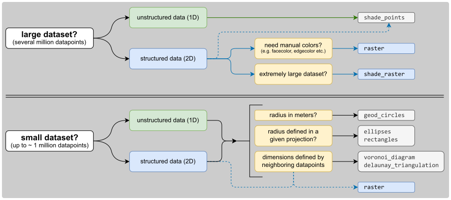
To specify how the data is represented on the map, you have to set the “plot-shape” via m.set_shape.

Note

Some “plot-shapes” require more computational effort than others!

Make sure to select an appropriate shape based on the size of the dataset you want to plot!

Maps.set_shape

Set the plot-shape to represent the data-points.

Possible shapes that work nicely for datasets with up to ~500 000 data-points:

`geod_circles`	Draw geodesic circles with a radius defined in meters.
`ellipses`	Draw projected ellipses with dimensions defined in units of a given crs.
`rectangles`	Draw projected rectangles with fixed dimensions (and possibly curved edges)
`voronoi_diagram`	Draw a Voronoi-Diagram of the data.
`delaunay_triangulation`	Draw a Delaunay-Triangulation of the data.

Possible shapes that work nicely for up to a few million data-points:

raster

Draw the data as a rectangular raster.

While raster can still be used for datasets with a few million datapoints, for extremely large datasets (> 10 million datapoints) it is recommended to use “shading” to greatly speed-up plotting. If shading is used, a dynamic averaging of the data based on the screen-resolution and the currently visible plot-extent is performed (resampling based on the mean-value is used by default).

Possible shapes that can be used to quickly generate a plot for extremely large datasets are:

`shade_points`	Shade the data as infinitesimal points (>> usable for very large datasets!).
`shade_raster`	Shade the data as a rectangular raster (>> usable for very large datasets!).

from eomaps import Maps
data, x, y = [.3,.64,.2,.5,1], [1,2,3,4,5], [2,5,3,7,5]

m = Maps()                                # create a Maps-object
m.set_data(data, x, y)                    # assign some data to the Maps-object
m.set_shape.rectangles(radius=1,          # represent the datapoints as 1x1 degree rectangles
                        radius_crs=4326)  # (in epsg=4326 projection)
m.plot_map(cmap="viridis", zorder=1)      # plot the data

m2 = m.new_layer()                        # create a new Maps-object on the same layer
m2.set_data(data, x, y)                   # assign another dataset to the new Maps object
m2.set_shape.geod_circles(radius=50000,   # draw geodetic circles with 50km radius
                        n=100)          # use 100 intermediate points to represent the shape
m2.plot_map(ec="k", cmap="Reds",          # plot the data
            zorder=2, set_extent=False)   # (and avoid resetting the plot-extent)

Note

The “shade”-shapes require the additional datashader dependency! You can install it via: mamba install -c conda-forge datashader

What’s used by default?

By default, the plot-shape is assigned based on the associated dataset.

For datasets with less than 500 000 pixels, m.set_shape.ellipses() is used.
For larger 2D datasets m.set_shape.shade_raster() is used

… and m.set_shape.shade_points() is used for the rest.

To get an overview of the existing shapes and their main use-cases, here’s a simple decision-tree:

🗺 Plot the map and save it

If you want to plot a map based on a dataset, first set the data and then call m.plot_map().

Any additional keyword-arguments passed to m.plot_map() are forwarded to the actual plot-command for the selected shape.

Some useful arguments that are supported by most shapes (except “shade”-shapes) are:

“cmap” : the colormap to use

“vmin”, “vmax” : the range of values used when assigning the colors

“fc” or “facecolor” : the face-color of the shapes

“ec” or “edgecolor” : the edge-color of the shapes

“lw” or “linewidth” : the linewidth of the shapes

“alpha” : the alpha-transparency

By default, the plot-extent of the axis is adjusted to the extent of the data. To keep the extent as-is, use m.plot_map(set_extent=False)

from eomaps import Maps
m = Maps()
m.add_feature.preset.coastline(lw=0.5)

m.set_data([1,2,3,4,5], [10,20,40,60,70], [10,20,50,70,30], crs=4326)
m.set_shape.geod_circles(radius=7e5)
m.plot_map(cmap="viridis", ec="b", lw=1.5, alpha=0.85, set_extent=False)

To adjust the margins of the subplots, use m.subplots_adjust, e.g.:

from eomaps import Maps
m = Maps()
m.subplots_adjust(left=0.1, right=0.9, bottom=0.05, top=0.95)

Maps.subplots_adjust

Update the subplot parameters of the grid.

You can then continue to add 🌈 Colorbars (with a histogram), 🏕 Annotations, Markers, Lines, Logos, etc., 📏 Scalebars, 🧭 Compass (or North Arrow), 🛰 WebMap layers, 🌵 NaturalEarth features or 💠 GeoDataFrames to the map, or you can start to ✏️ Draw Shapes on the map, add 🦜 Utility widgets and 🛸 Callbacks - make the map interactive!.

Once the map is ready, an image of the map can be saved at any time by using:

m.savefig( "snapshot1.png", dpi=300, ... )

`Maps.plot_map`	Actually generate the map-plot based on the data provided as m.data and the specifications defined in "data_specs" and "classify_specs".
`Maps.savefig`	Save the current figure.

🎨 Customizing the plot

All arguments to customize the appearance of a dataset are passed to m.plot_map(...).

In general, the colors assigned to the shapes are specified by

selecting a colormap (cmap)
- either a name of a pre-defined matplotlib colormap (e.g. "viridis", "RdYlBu" etc.)
- or a general matplotlib colormap object (see matplotlib-docs for more details)
(optionally) setting appropriate data-limits via vmin and vmax.
- vmin and vmax set the range of data-values that are mapped to the colorbar-colors
- Any values outside this range will get the colormaps over and under colors assigned.

m = Maps()
m.set_data(...)
m.plot_map(cmap="viridis", vmin=0, vmax=1)

Colors can also be set manually by providing one of the following arguments to m.plot_map(...):

to set both facecolor AND edgecolor use color=...
to set the facecolor use fc=... or facecolor=...
to set the edgecolor use ec=... or edgecolor=...

Note

Manual color specifications do not work with the shade_raster and shade_points shapes!
Providing manual colors will override the colors assigned by the cmap!
The colorbar does not represent manually defined colors!

Uniform colors

To apply a uniform color to all datapoints, you can use matpltolib’s color-names or pass an RGB or RGBA tuple.

m.plot_map(fc="r")
m.plot_map(fc="orange")
m.plot_map(fc=(1, 0, 0.5))
m.plot_map(fc=(1, 0, 0.5, .25))
# for grayscale use a string of a number between 0 and 1
m.plot_map(fc="0.3")

Explicit colors

To explicitly color each datapoint with a pre-defined color, simply provide a list or array of the aforementioned types.

m.plot_map(fc=["r", "g", "orange"])
# for grayscale use a string of a number between 0 and 1
m.plot_map(fc=[".1", ".2", "0.3"])
# or use RGB / RGBA tuples
m.plot_map(fc=[(1, 0, 0.5), (.3, .4, .5), (1, 1, 0)])
m.plot_map(fc=[(1, 0, 0.5, .25), (1, 0, 0.5, .75), (.1, .2, 0.5, .5)])

RGB composites

To create an RGB or RGBA composite from 3 (or 4) datasets, pass the datasets as tuple:

the datasets must have the same size as the coordinate arrays!
the datasets must be scaled between 0 and 1

# if you pass a tuple of 3 or 4 arrays, they will be used to set the
# RGB (or RGBA) colors of the shapes
m.plot_map(fc=(<R-array>, <G-array>, <B-array>))
m.plot_map(fc=(<R-array>, <G-array>, <B-array>, <A-array>))

# you can fix individual color channels by passing a list with 1 element
m.plot_map(fc=(<R-array>, [0.12345], <B-array>, <A-array>))

📊 Data classification

EOmaps provides an interface for mapclassify to classify datasets prior to plotting.

There are 2 (synonymous) ways to assign a classification-scheme:

m.set_classify_specs(scheme=..., ...): set classification scheme by providing name and relevant parameters.
m.set_classify.<SCHEME>(...): use autocompletion to get available classification schemes (with appropriate docstrings)
- The big advantage of this method is that it supports autocompletion (once the Maps-object has been instantiated) and provides relevant docstrings to get additional information on the classification schemes.

Available classifier names are also accessible via Maps.CLASSIFIERS.

The preferred way for assigning a classification-scheme to a Maps object is:

m = Maps()
m.set_data(...)
m.set_shape.ellipses(...)
m.set_classify.Quantiles(k=5)
m.plot_map()

Alternatively, one can also use m.set_classify_specs to assign a classification scheme:

m = Maps()
m.set_data(...)
m.set_shape.ellipses(...)

m.set_classify_specs(scheme="Quantiles", k=5)
m.classify_specs.k = 10 # alternative way for setting classify-specs
m.plot_map()

`Maps.set_classify`
`Maps.set_classify_specs`	Set classification specifications for the data.

Currently available classification-schemes are (see mapclassify for details):

BoxPlot (hinge)
EqualInterval (k)
FisherJenks (k)
FisherJenksSampled (k, pct, truncate)
HeadTailBreaks ()
JenksCaspall (k)
JenksCaspallForced (k)
JenksCaspallSampled (k, pct)
MaxP (k, initial)
MaximumBreaks (k, mindiff)
NaturalBreaks (k, initial)
Quantiles (k)
Percentiles (pct)
StdMean (multiples)
UserDefined (bins)

🍱 Adding Maps to existing figures

It is possible to add (one or more) EOmaps maps to existing matplotlib figures.

To create a new map in an existing figure, simply provide the matplotlib.Figure instance via Maps(f=<the figure instance>)
The initial position of the map can be set via the ax argument, e.g.: Maps(ax=<...>).
- NOTE: Since the effective size of the Map is dependent on the current zoom-region, the position always represents the maximal area that can be occupied by the map!

The syntax is similar to matplotlibs f.add_subplot() or f.add_axes, allowing one of the following options:

Grid positioning

To position the map in a (virtual) grid, one of the following options are possible:

Three integers (nrows, ncols, index).
- The map will take the index position on a grid with nrows rows and ncols columns.
- index starts at 1 in the upper left corner and increases to the right.
- index can also be a two-tuple specifying the (first, last) indices (1-based, and including last) of the map, e.g., Maps(ax=(3, 1, (1, 2))) makes a map that spans the upper 2/3 of the figure.

import matplotlib.pyplot as plt
from eomaps import Maps

f = plt.figure(figsize=(10, 7))  # initialize the Figure
f.add_subplot(2, 2, 1)           # add a normal axes
m = Maps(f=f, ax=(2, 2, (1, 2))) # add a EOmaps map

f = plt.figure(figsize=(10, 7))  # initialize the Figure
f.add_subplot(3, 1, 1)           # add a normal axes
m = Maps(f=f, ax=(3, 1, (2, 3))) # add a EOmaps map

A 3-digit integer.
- The digits are interpreted as if given separately as three single-digit integers, i.e. Maps(ax=235) is the same as Maps(ax=(2, 3, 5)).
- Note that this can only be used if there are no more than 9 subplots.

import matplotlib.pyplot as plt
from eomaps import Maps

f = plt.figure(figsize=(10, 7)) # initialize the Figure
f.add_subplot(211)              # add a normal axes
m = Maps(f=f, ax=212)           # add a EOmaps map

An already existing matplotlib.Axes instance
- NOTE: this MUST be a cartopy-GeoAxes with the same projection as the Maps-object!

import matplotlib.pyplot as plt
import cartopy
from eomaps import Maps

f = plt.figure(figsize=(10, 7))   # initialize the Figure
ax = f.add_subplot(projection=cartopy.crs.Mollweide())
m = Maps(ax=ax)

A matplotlib.SubplotSpec

import matplotlib.pyplot as plt
from matplotlib.gridspec import GridSpec
from eomaps import Maps

gs = GridSpec(2, 2)              # setup the GridSpec

f = plt.figure(figsize=(10, 7))  # initialize the Figure
m = Maps(f=f, ax=gs[0,0])        # add a EOmaps map

Absolute positioning

To set the absolute position of the map, provide a list of 4 floats representing (left, bottom, width, height).

The absolute position of the map expressed in relative figure coordinates (e.g. ranging from 0 to 1)

import matplotlib.pyplot as plt
from eomaps import Maps

f = plt.figure(figsize=(10, 7))   # initialize the Figure
f.add_axes((.2, .5, .4, .4))      # add a normal axes
m = Maps(f=f, ax=(.2, 0, .4, .5)) # add a EOmaps map

Dynamic updates of plots

As soon as a Maps-object is attached to a figure, EOmaps will handle re-drawing of the figure. Therefore dynamically updated artists must be added to the “blit-manager” (m.BM) to ensure that they are correctly updated.

use m.BM.add_artist(artist, layer=...) if the artist should be re-drawn on any change in the figure
use m.BM.add_bg_artist(artist, layer=...) if the artist should only be re-drawn if the extent of the map changes

In general, it should be sufficient to simply add the axes-object as artist via m.BM.add_artist(...) This will ensure that all artists on the axes are updated.

Here’s a more complete example to show how it works:

import matplotlib.pyplot as plt
from eomaps import Maps

# create a matplotlib figure
f = plt.figure(figsize=(10, 7))
# add a "normal" plot spanning the top rows of a 2x2 grid
ax = f.add_subplot(2, 2, (1, 2))
ax.plot([10, 20, 30, 40, 50], [10, 20, 30, 40, 50])

# put a map on the 3rd axis of a 2x2 grid (bottom left)
m = Maps(f=f, ax=(2, 2, 3))
m.ax.set_title("click me!")
m.add_wms.OpenStreetMap.add_layer.default()
m.cb.click.attach.mark(radius=20, fc="none", ec="r", lw=2)

# attach a callback that plots markers on the axis if you click on the map
def cb(pos, **kwargs):
    ax.plot(*pos, marker="o")
m.cb.click.attach(cb)

# Since we want to dynamically update the plot on the axis, it must be
# added to the BlitManager to ensure that the artists are properly updated.
# (EOmaps handles interactive re-drawing of the figure)
m.BM.add_artist(ax, layer=m.layer)

# put a map on the 4th axis of a 2x2 grid (bottom right)
m2 = Maps(f=f, ax=(2, 2, 4), crs=Maps.CRS.Mollweide())
m2.add_feature.preset.coastline()
m2.add_feature.preset.ocean()
m2.cb.click.attach.mark(radius=20, fc="none", ec="r", lw=2, n=200)

# share click events on the 2 maps
m.cb.click.share_events(m2)

𝄜 MapsGrid objects

MapsGrid objects can be used to create (and manage) multiple maps in one figure.

A MapsGrid creates a grid of Maps objects (and/or ordinary matpltolib axes), and provides convenience-functions to perform actions on all maps of the figure.

from eomaps import MapsGrid
mg = MapsGrid(r=2, c=2, crs=..., layer=..., ... )
# you can then access the individual Maps-objects via:
mg.m_0_0
mg.m_0_1
mg.m_1_0
mg.m_1_1

m2 = mg.m_0_0.new_layer("newlayer")
...

# there are many convenience-functions to perform actions on all Maps-objects:
mg.add_feature.preset.coastline()
mg.add_compass()
...

# to perform more complex actions on all Maps-objects, simply loop over the MapsGrid object
for m in mg:
    ...

# set the margins of the plot-grid
mg.subplots_adjust(left=0.1, right=0.9, bottom=0.05, top=0.95, hspace=0.1, wspace=0.05)

Make sure to checkout the 🏗️ Layout Editor which greatly simplifies the arrangement of multiple axes within a figure!

Custom grids and mixed axes

Fully customized grid-definitions can be specified by providing m_inits and/or ax_inits dictionaries of the following structure:

The keys of the dictionary are used to identify the objects
The values of the dictionary are used to identify the position of the associated axes
The position can be either an integer N, a tuple of integers or slices (row, col)
Axes that span over multiple rows or columns, can be specified via slice(start, stop)

dict(
    name1 = N  # position the axis at the Nth grid cell (counting firs)
    name2 = (row, col), # position the axis at the (row, col) grid-cell
    name3 = (row, slice(col_start, col_end)) # span the axis over multiple columns
    name4 = (slice(row_start, row_end), col) # span the axis over multiple rows
    )

m_inits is used to initialize Maps objects
ax_inits is used to initialize ordinary matplotlib axes

The individual Maps-objects and matpltolib-Axes are then accessible via:

mg = MapsGrid(2, 3,
              m_inits=dict(left=(0, 0), right=(0, 2)),
              ax_inits=dict(someplot=(1, slice(0, 3)))
              )
mg.m_left   # the Maps object with the name "left"
mg.m_right   # the Maps object with the name "right"

mg.ax_someplot   # the ordinary matplotlib-axis with the name "someplot"

❗ NOTE: if m_inits and/or ax_inits are provided, ONLY the explicitly defined objects are initialized!

The initialization of the axes is based on matplotlib’s GridSpec functionality. All additional keyword-arguments (width_ratios, height_ratios, etc.) are passed to the initialization of the GridSpec object.
To specify unique crs for each Maps object, provide a dictionary of crs specifications.

from eomaps import MapsGrid

# initialize a grid with 2 Maps objects and 1 ordinary matplotlib axes
mgrid = MapsGrid(2, 2,
                 m_inits=dict(top_row=(0, slice(0, 2)),
                              bottom_left=(1, 0)),
                 crs=dict(top_row=4326,
                          bottom_left=3857),
                 ax_inits=dict(bottom_right=(1, 1)),
                 width_ratios=(1, 2),
                 height_ratios=(2, 1))

mgrid.m_top_row # a map extending over the entire top-row of the grid (in epsg=4326)
mgrid.m_bottom_left # a map in the bottom left corner of the grid (in epsg=3857)

mgrid.ax_bottom_right # an ordinary matplotlib axes in the bottom right corner of the grid

`MapsGrid`	Initialize a grid of Maps objects
`MapsGrid.join_limits`	Join axis limits between all Maps objects of the grid (only possible if all maps share the same crs!)
`MapsGrid.share_click_events`	Share click events between all Maps objects of the grid
`MapsGrid.share_pick_events`	Share pick events between all Maps objects of the grid
`MapsGrid.set_data_specs`	This will execute the corresponding action on ALL Maps objects of the MapsGrid!
`MapsGrid.set_classify_specs`	This will execute the corresponding action on ALL Maps objects of the MapsGrid!
`MapsGrid.add_wms`	A collection of open-access WebMap services that can be added to the maps.
`MapsGrid.add_feature`	Interface to the feature-layers provided by NaturalEarth.
`MapsGrid.add_annotation`	This will execute the corresponding action on ALL Maps objects of the MapsGrid!
`MapsGrid.add_marker`	This will execute the corresponding action on ALL Maps objects of the MapsGrid!
`MapsGrid.add_gdf`	This will execute the corresponding action on ALL Maps objects of the MapsGrid!

🧱 Naming conventions and autocompletion

The goal of EOmaps is to provide a comprehensive, yet easy-to-use interface.

To avoid having to remember a lot of names, a concise naming-convention is applied so that autocompletion can quickly narrow-down the search to relevant functions and properties.

Once a few basics keywords have been remembered, finding the right functions and properties should be quick and easy.

Note

EOmaps works best in conjunction with “dynamic autocompletion”, e.g. by using an interactive console where you instantiate a Maps object first and then access dynamically updated properties and docstrings on the object.

To clarify:

First, execute m = Maps() in an interactive console
then (inside the console, not inside the editor!) use autocompletion on m. to get autocompletion for dynamically updated attributes.

For example the following accessors only work properly after the Maps object has been initialized: - m.add_wms: browse available WebMap services - m.set_classify: browse available classification schemes

The following list provides an overview of the naming-conventions used within EOmaps:

Add features to a map - “m.add_”

All functions that add features to a map start with add_, e.g.: - m.add_feature, m.add_wms, m.add_annotation, m.add_marker, m.add_gdf, …

WebMap services (e.g. m.add_wms) are fetched dynamically from the respective APIs. Therefore the structure can vary from one WMS to another. The used convention is the following: - You can navigate into the structure of the API by using “dot-access” continuously - once you reach a level that provides layers that can be added to the map, the .add_layer. directive will be visible - any <LAYER> returned by .add_layer.<LAYER> can be added to the map by simply calling it, e.g.:

m.add_wms.OpenStreetMap.add_layer.default()

m.add_wms.OpenStreetMap.OSM_mundialis.add_layer.OSM_WMS()

Set data specifications - “m.set_”

All functions that set properties of the associated dataset start with set_, e.g.: - m.set_data, m.set_classify, m.set_shape, …

Create new Maps-objects - “m.new_”

Actions that result in a new Maps objects start with new_. - m.new_layer, m.new_inset_map, …

Callbacks - “m.cb.”

Everything related to callbacks is grouped under the cb accessor.

use m.cb.<METHOD>.attach.<CALLBACK>() to attach pre-defined callbacks
- <METHOD> hereby can be one of click, pick or keypress (but there’s no need to remember since autocompletion will do the job!).
use m.cb.<METHOD>.attach(custom_cb) to attach a custom callback

🧰 Companion Widget

Starting with v5.0, EOmaps comes with an awesome companion widget that greatly simplifies using interactive capabilities.

To activate the widget, press w on the keyboard while the mouse is over the map you want to edit.
- If multiple maps are present in the figure, a green border indicates the map that is currently targeted by the widget.
- Once the widget is initialized, pressing w will show/hide the widget.

What are the buttons and sliders doing?

To get information on how the individual controls work, simply click on the ? symbol in the top left corner of the widget!

This will activate help tooltips that explain the individual controls.

Note

The companion-widget is written in PyQt5 and therefore only works when using the matplotlib qt5agg backend (matplotlibs default if QT5 is installed)!

To manually set the backend, execute the following lines at the start of your script:

import matplotlib
matplotlib.use("qt5agg")

The main purpose of the widget is to provide easy-access to features that usually don’t need to go into a python-script, such as:

Compare layers (e.g. overlay multiple layers)
Switch between existing layers (or combine existing layers)
Add simple click or pick callbacks
Quickly create new WebMap layers (or add WebMap services to existing layers)
Draw shapes, add Annotations and NaturalEarth features to the map
Quick-edit existing map-artists (show/hide, remove or set basic properties color, linewidth, zorder)
Save the current state of the map to a file (at the desired dpi setting)
A basic interface to plot data from files (with drag-and-drop support) (csv, NetCDF, GeoTIFF, shapefile)

🛸 Callbacks - make the map interactive!

Callbacks are used to execute functions when you click on the map.

They can be attached to a map via the .attach directive:

m = Maps()
...
m.cb.< METHOD >.attach.< CALLBACK >( **kwargs )

< METHOD > defines the way how callbacks are executed.

`click`	Callbacks that are executed if you click anywhere on the Map.
`pick`	Callbacks that select the nearest datapoint(s) if you click on the map.
`move`	Callbacks that are executed if you press a key on the keyboard.
`keypress`	Callbacks that are executed if you move the mouse without holding down a button.

< CALLBACK > indicates the action you want to assign to the event. There are many pre-defined callbacks, but it is also possible to define custom functions and attach them to the map (see below).

from eomaps import Maps
import numpy as np
x, y = np.mgrid[-45:45, 20:60]

m = Maps(Maps.CRS.Orthographic())
m.all.add_feature.preset.coastline()
m.set_data(data=x+y**2, x=x, y=y, crs=4326)
m.plot_map(pick_distance=10)

m2 = m.new_layer(copy_data_specs=True, layer="second_layer")
m2.plot_map(cmap="tab10")

# get an annotation if you RIGHT-click anywhere on the map
m.cb.click.attach.annotate(xytext=(-60, -60),
                           bbox=dict(boxstyle="round", fc="r"))

# pick the nearest datapoint if you click on the MIDDLE mouse button
m.cb.pick.attach.annotate(button=2)
m.cb.pick.attach.mark(buffer=1, permanent=False, fc="none", ec="r", button=2)
m.cb.pick.attach.mark(buffer=4, permanent=False, fc="none", ec="r", button=2)

# peek at the second layer if you LEFT-click on the map
m.cb.click.attach.peek_layer("second_layer", how=.25, button=3)

Note

Callbacks are only executed if the layer of the associated Maps object is actually visible! (This assures that pick-callbacks always refer to the visible dataset.)

To define callbacks that are executed independent of the visible layer, attach it to the "all" layer using something like m.all.cb.click.attach.annotate().

In addition, each callback-container supports the following useful methods:

`attach`	Attach custom or pre-defined callbacks to the map.
`remove`	Remove previously attached callbacks from the map.
`get`	Accessor for objects generated/retrieved by callbacks.
`set_sticky_modifiers`	Define keys on the keyboard that should be treated as “sticky modifiers”.

`share_events`	Share callback-events between this Maps-object and all other Maps-objects
`forward_events`	Forward callback-events from this Maps-object to other Maps-objects
`add_temporary_artist`	Make an artist temporary (remove it from the map at the next event)

🍬 Pre-defined callbacks

Pre-defined click, pick and move callbacks

Callbacks that can be used with m.cb.click, m.cb.pick and m.cb.move:

`peek_layer`	Swipe between data- or WebMap layers or peek a layers through a rectangle.
`annotate`	Add a basic text-annotation to the plot at the position where the map was clicked.
`mark`	Draw markers at the location where the map was clicked.
`print_to_console`	Print details on the clicked pixel to the console

Callbacks that can be used with m.cb.click and m.cb.pick:

`get_values`	Successively collect return-values in a dict accessible via m.cb.[click/pick].get.picked_vals.
`clear_annotations`	Remove all temporary and permanent annotations from the plot
`clear_markers`	Remove all temporary and permanent annotations from the plot.

Callbacks that can be used only with m.cb.pick:

`load`	Load objects from a given database using the ID of the picked pixel.
`highlight_geometry`	Temporarily highlite the picked geometry of a GeoDataFrame.

Pre-defined keypress callbacks

Callbacks that can be used with m.cb.keypress

`switch_layer`	Change the default layer of the map.
`fetch_layers`	Fetch (and cache) layers of a map.

👽 Custom callbacks

Custom callback functions can be attached to the map via m.cb.< METHOD >.attach(< CALLBACK FUNCTION >, **kwargs):

def some_callback(custom_kwarg, **kwargs):
    print("the value of 'custom_kwarg' is", custom_kwarg)
    print("the position of the clicked pixel in plot-coordinates", kwargs["pos"])
    print("the dataset-index of the nearest datapoint", kwargs["ID"])
    print("data-value of the nearest datapoint", kwargs["val"])
    print("the color of the nearest datapoint", kwargs["val_color"])
    print("the numerical index of the nearest datapoint", kwargs["ind"])
    ...

# attaching custom callbacks works completely similar for "click", "pick" and "keypress"!
m = Maps()
...
m.cb.pick.attach(some_callback, double_click=False, button=1, custom_kwarg=1)
m.cb.click.attach(some_callback, double_click=False, button=2, custom_kwarg=2)
m.cb.keypress.attach(some_callback, key="x", custom_kwarg=3)

Note

Custom callbacks must always accept the following keyword arguments: pos, ID, val, val_color, ind

❗ for click callbacks the kwargs ID, val and val_color are set to None!
❗ for keypress callbacks the kwargs ID, val, val_color, ind and pos are set to None!

For better readability it is recommended that you “unpack” used arguments like this:

def cb(ID, val, **kwargs):
    print(f"the ID is {ID} and the value is {val}")

👾 Using modifiers for pick- click- and move callbacks

It is possible to trigger pick, click or move callbacks only if a specific key is pressed on the keyboard.

This is achieved by specifying a modifier when attaching a callback, e.g.:

m = Maps()
m.add_feature.preset.coastline()
# a callback that is executed if NO modifier is pressed
m.cb.move.attach.mark(radius=5)
# a callback that is executed if 1 is pressed while moving the mouse
m.cb.move.attach.mark(modifier="1", radius=10, fc="r", ec="g")
# a callback that is executed if 2 is pressed while moving the mouse
m.cb.move.attach.mark(modifier="2", radius=15, fc="none", ec="b")

To keep the last pressed modifier active until a new modifier is activated, you can make it “sticky” by using m.cb.move.set_sticky_modifiers().

“Sticky modifiers” remain activated until
- A new (sticky) modifier is activated
- ctrl + <current (sticky) modifier> is pressed
- escape is pressed

NOTE: sticky modifiers are defined for each callback method individually! (e.g. sticky modifiers are unique for click, pick and move callbacks)

m = Maps()
m.add_feature.preset.coastline()

# a callback that is executed if 1 is pressed while clicking on the map
m.cb.click.attach.annotate(modifier="1", text="modifier 1 active")
# a callback that is executed if 2 is pressed while clicking on the map
m.cb.click.attach.annotate(modifier="2", text="modifier 2 active")

# make the modifiers 1 and 2 sticky for click callbacks
m.cb.click.set_sticky_modifiers("1", "2")

# note that the modifier 1 is not sticky for move callbacks!
# m.cb.move.set_sticky_modifiers("1")  # (uncomment to make it sticky)
m.cb.move.attach.mark(radius=5)
m.cb.move.attach.mark(modifier="1", radius=5, fc="r")

🍭 Picking N nearest neighbours

[requires EOmaps >= 5.4]

By default pick-callbacks pick the nearest datapoint with respect to the click position.

To customize the picking-behavior, use m.cb.pick.set_props(). The following properties can be adjusted:

n: The (maximum) number of datapoints to pick within the search-circle.
search_radius: The radius of a circle (in units of the plot-crs) that is used to identify the nearest neighbours.
pick_relative_to_closest: Set the center of the search-circle.
- If True, the nearest neighbours are searched relative to the closest identified datapoint.
- If False, the nearest neighbours are searched relative to the click position.
consecutive_pick: Pick datapoints individually or alltogether.
- If True, callbacks are executed for each picked point individually
- If False, callbacks are executed only once and get lists of all picked values as input-arguments.

set_props

Set the picker-properties (number of picked points, max.

from eomaps import Maps
import numpy as np

# create some random data
x, y = np.mgrid[-30:67, -12:50]
data = np.random.randint(0, 100, x.shape)

# a callback to indicate the search-radius
def indicate_search_radius(m, pos, *args, **kwargs):
    art = m.add_marker(
        xy=(np.atleast_1d(pos[0])[0],
            np.atleast_1d(pos[1])[0]),
        shape="ellipses", radius=m.tree.d, radius_crs="out",
        n=100, fc="none", ec="k", lw=2)
    m.cb.pick.add_temporary_artist(art)

# a callback to set the number of picked neighbours
def pick_n_neighbours(m, n, **kwargs):
    m.cb.pick.set_props(n=n)


m = Maps()
m.add_feature.preset.coastline()
m.set_data(data, x, y)
m.plot_map()
m.cb.pick.set_props(n=50, search_radius=10, pick_relative_to_closest=True)

m.cb.pick.attach.annotate()
m.cb.pick.attach.mark(fc="none", ec="r")
m.cb.pick.attach(indicate_search_radius, m=m)

for key, n in (("1", 1), ("2", 9), ("3", 50), ("4", 500)):
    m.cb.keypress.attach(pick_n_neighbours, key=key, m=m, n=n)

📍 Picking a dataset without plotting it first

It is possible to attach pick callbacks to a Maps object without plotting the data first by using m.make_dataset_pickable().

m = Maps()
m.add_feature.preset.coastline()
m.set_data(... the dataset ...)
m.make_dataset_pickable()
# now it's possible to attach pick-callbacks even though the data is still "invisible"
m.cb.pick.attach.annotate()

Note

Using m.make_dataset_pickable() is ONLY necessary if you want to use pick callbacks without actually plotting the data! Otherwise a call to m.plot_map() is sufficient!

make_dataset_pickable

Make the associated dataset pickable without plotting it first.

🛰 WebMap layers

WebMap services (TS/WMS/WMTS) can be attached to the map via:

m.add_wms.attach.< SERVICE > ... .add_layer.< LAYER >(...)

< SERVICE > hereby specifies the pre-defined WebMap service you want to add, and < LAYER > indicates the actual layer-name.

m = Maps(Maps.CRS.GOOGLE_MERCATOR) # (the native crs of the service)
m.add_wms.OpenStreetMap.add_layer.default()

Maps.add_wms

A collection of open-access WebMap services that can be added to the maps.

Note

It is highly recommended (and sometimes even required) to use the native crs of the WebMap service in order to avoid re-projecting the images (which degrades image quality and sometimes takes quite a lot of time to finish…)

most services come either in epsg=4326 or in Maps.CRS.GOOGLE_MERCATOR projection

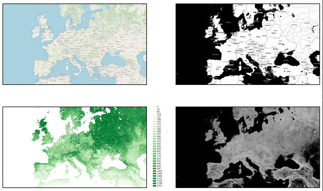
from eomaps import Maps, MapsGrid
mg = MapsGrid(crs=Maps.CRS.GOOGLE_MERCATOR)
mg.join_limits()

mg.m_0_0.add_wms.OpenStreetMap.add_layer.default()
mg.m_0_1.add_wms.OpenStreetMap.add_layer.stamen_toner()

mg.m_1_1.add_wms.S1GBM.add_layer.vv()

# ... for more advanced
layer = mg.m_1_0.add_wms.ISRIC_SoilGrids.nitrogen.add_layer.nitrogen_0_5cm_mean
layer.set_extent_to_bbox() # set the extent according to the boundingBox
layer.info                 # the "info" property provides useful information on the layer
layer()                    # call the layer to add it to the map
layer.add_legend()         # if a legend is provided, you can add it to the map!

Pre-defined WebMap services:

Global:

`OpenStreetMap`	OpenStreetMap WebMap layers https://wiki.openstreetmap.org/wiki/WMS
`ESA_WorldCover`	ESA Worldwide land cover mapping https://esa-worldcover.org/en
`NASA_GIBS`	NASA Global Imagery Browse Services (GIBS) https://wiki.earthdata.nasa.gov/display/GIBS/
`ISRIC_SoilGrids`	Interface to the ISRIC SoilGrids database.
`EEA_DiscoMap`	European Environment Agency Discomap services https://discomap.eea.europa.eu/Index/
`ESRI_ArcGIS`	Interface to the ERSI ArcGIS REST Services Directory http://services.arcgisonline.com/arcgis/rest/services
`S1GBM`	Sentinel-1 Global Backscatter Model https://researchdata.tuwien.ac.at/records/n2d1v-gqb91
`S2_cloudless`	Global cloudless Sentinel-2 maps, crafted by EOX https://s2maps.eu/
`GEBCO`	Global ocean & land terrain models https://www.gebco.net/
`CAMS`	Copernicus Atmosphere Monitoring Service (Global and European) https://atmosphere.copernicus.eu/
`DLR_basemaps`	Basemaps hosted by DLR's EOC Geoservice https://geoservice.dlr.de

Services specific for Austria (Europe)

`Austria.AT_basemap`	Basemap for Austria https://basemap.at/
`Austria.Wien_basemap`	Basemaps for the city of Vienna (Austria) https://www.wien.gv.at

Note

Services might be nested directory structures! The actual layer is always added via the add_layer directive.

m.add_wms.<...>. ... .<...>.add_layer.<LAYER NAME>()

Some of the services dynamically fetch the structure via HTML-requests. Therefore it can take a short moment before autocompletion is capable of showing you the available options! A list of available layers from a sub-folder can be fetched via:

m.add_wms.<...>. ... .<LAYER NAME>.layers

Using custom WebMap services

It is also possible to use custom WMS/WMTS/XYZ services. (see docstring of m.add_wms.get_service for more details and examples)

get_service

Get a object that can be used to add WMS, WMTS or XYZ services based on a GetCapabilities-link or a link to a ArcGIS REST API

m = Maps()
# define the service
service = m.add_wms.get_service(<... link to GetCapabilities.xml ...>,
                                service_type="wms",
                                res_API=False,
                                maxzoom=19)
# once the service is defined, you can use it just like the pre-defined ones
service.layers   # >> get a list of all layers provided by the service

# select one of the layers
layer = service.add_layer. ... .< LAYER >
layer.info                  # >> get some additional infos for the selected layer
layer.set_extent_to_bbox()  # >> set the map-extent to the bbox of the layer

# call the layer to add it to the map
# (optionally providing additional kwargs for fetching map-tiles)
layer(...)

Setting date, style and other WebMap properties

Some WebMap services allow passing additional arguments to set properties such as the date or the style of the map. To pass additional arguments to a WebMap service, simply provide them when when calling the layer, e.g.:

m = Maps()
m.add_wms.< SERVICE >. ... .add_layer.< LAYER >(time=..., styles=[...], ...)

To show an example, here’s how to fetch multiple timestamps for the UV-index of the Copernicus Airquality service. (provided by https://atmosphere.copernicus.eu/)

from eomaps import Maps
import pandas as pd

m = Maps(layer="all", figsize=(8, 4))
m.subplots_adjust(left=0.05, right=0.95)
m.all.add_feature.preset.coastline()
m.add_logo()

layer = m.add_wms.CAMS.add_layer.composition_uvindex_clearsky
timepos = layer.wms_layer.timepositions   # available time-positions
all_styles = list(layer.wms_layer.styles) # available styles

# create a list of timestamps to fetch
start, stop, freq = timepos[1].split(r"/")
times = pd.date_range(start, stop, freq=freq.replace("PT", ""))
times = times.strftime("%Y-%m-%dT%H:%M:%SZ")

style = all_styles[0]     # use the first available style
for time in times[:6]:
    # call the layer to add it to the map
    layer(time=time,
          styles=[style],   # provide a list with 1 entry here
          layer=time        # put each WebMap on an individual layer
          )

layer.add_legend()  # add a legend for the WebMap service

# add a "slider" and a "selector" widget
m.util.layer_selector(ncol=3, loc="upper center", fontsize=6, labelspacing=1.3)
m.util.layer_slider()

# attach a callback to fetch all layers if you press l on the keyboard
cid = m.all.cb.keypress.attach.fetch_layers(key="l")
# fetch all layers so that they are cached and switching layers is fast
m.fetch_layers()
m.show_layer(times[0])      # make the first timestamp visible

🌵 NaturalEarth features

Feature-layers provided by NaturalEarth can be directly added to the map via m.add_feature.

Maps.add_feature

Interface to the feature-layers provided by NaturalEarth.

The call-signature is: m.add_feature.< CATEGORY >.< FEATURE >(...):

< CATEGORY > specifies the general category of the feature, e.g.:

cultural: cultural features (e.g. countries, states etc.)
physical: physical features (e.g. coastlines, land, ocean etc.)
preset: a set of pre-defined layers for convenience (see below)

< FEATURE > is the name of the NaturalEarth feature, e.g. "coastlines", "admin_0_countries" etc..

from eomaps import Maps
m = Maps()
m.add_feature.preset.coastline()
m.add_feature.preset.ocean()
m.add_feature.preset.land()
m.add_feature.preset.countries()

m.add_feature.physical.lakes(scale=110, ec="b")
m.add_feature.cultural.admin_0_pacific_groupings(ec="m", lw=2)

# (only if geopandas is installed)
places = m.add_feature.cultural.populated_places.get_gdf(scale=110)
m.add_gdf(places, markersize=places.NATSCALE/10, fc="r")

NaturalEarth provides features in 3 different scales: 1:10m, 1:50m, 1:110m. By default EOmaps uses features at 1:50m scale. To set the scale manually, simply use the scale argument when calling the feature.

It is also possible to automatically update the scale based on the map-extent by using scale="auto". (Note that if you zoom into a new scale the data might need to be downloaded and reprojected so the map might be irresponsive for a couple of seconds until everything is properly cached.)

If you want to get a geopandas.GeoDataFrame containing all shapes and metadata of a feature, use: (Have a look at 💠 GeoDataFrames on how to add the obtained GeoDataFrame to the map)

from eomaps import Maps
m = Maps()
gdf = m.add_feature.physical.coastline.get_gdf(scale=10)

The most commonly used features are accessible with pre-defined colors via the preset category:

`coastline`	Add a coastline to the map.
`ocean`	Add ocean-coloring to the map.
`land`	Add a land-coloring to the map.
`countries`	Add country-boundaries to the map.
`urban_areas`	Add urban-areas to the map.
`lakes`	Add lakes to the map.
`rivers_lake_centerlines`	Add rivers_lake_centerlines to the map.

💠 GeoDataFrames

A geopandas.GeoDataFrame can be added to the map via m.add_gdf().

This is basically just a wrapper for the plotting capabilities of geopandas (e.g. gdf.plot(...) ) supercharged with EOmaps features.

Maps.add_gdf

Plot a geopandas.GeoDataFrame on the map.

from eomaps import Maps
import geopandas as gpd

gdf = gpd.GeoDataFrame(geometries=[...], crs=...)<>

m = Maps()
m.add_gdf(gdf, fc="r", ec="g", lw=2)

It is possible to make the shapes of a GeoDataFrame pickable (e.g. usable with m.cb.pick callbacks) by providing a picker_name (and specifying a pick_method).

use pick_method="contains" if your GeoDataFrame consists of polygon-geometries (the default)
- pick a geometry if geometry.contains(mouse-click-position) == True
use pick_method="centroids" if your GeoDataFrame consists of point-geometries
- pick the geometry with the closest centroid

Once the picker_name is specified, pick-callbacks can be attached via:

m.cb.pick[<PICKER NAME>].attach.< CALLBACK >()

For example, to highlight the clicked country, you could use:

from eomaps import Maps
m = Maps()
# get the GeoDataFrame for a given NaturalEarth feature
gdf = m.add_feature.cultural_110m.admin_0_countries.get_gdf()

# pick the shapes of the GeoDataFrame based on a "contains" query
m.add_gdf(gdf, picker_name="countries", pick_method="contains")

# temporarily highlight the picked geometry
m.cb.pick["countries"].attach.highlight_geometry(fc="r", ec="g", lw=2)

🏕 Annotations, Markers, Lines, Logos, etc.

🔴 Markers

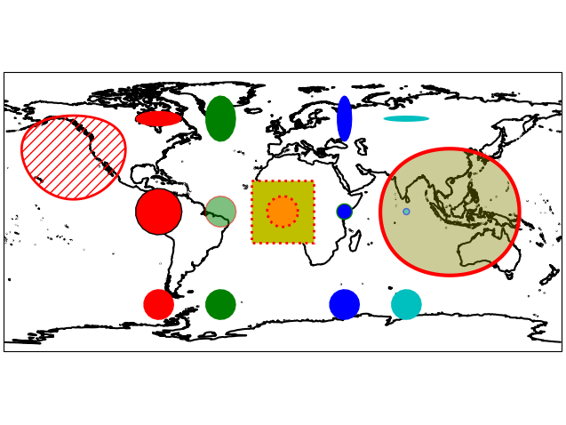
Static markers can be added to the map via m.add_marker().

If a dataset has been plotted, you can mark any datapoint via its ID, e.g. ID=...
To add a marker at an arbitrary position, use xy=(...)
- By default, the coordinates are assumed to be provided in the plot-crs
- You can specify arbitrary coordinates via xy_crs=...
The radius is defined via radius=...
- By default, the radius is assumed to be provided in the plot-crs
- You can specify the radius in an arbitrary crs via radius_crs=...
The marker-shape is set via shape=...
- Possible arguments are "ellipses", "rectangles", "geod_circles"
Additional keyword-arguments are passed to the matplotlib collections used to draw the shapes (e.g. “facecolor”, “edgecolor”, “linewidth”, “alpha”, etc.)
Multiple markers can be added in one go by using lists for xy, radius, etc.

🛸 For dynamic markers checkout m.cb.click.attach.mark() or m.cb.pick.attach.mark()

add_marker

add a marker to the plot

from eomaps import Maps
m = Maps(crs=4326)
m.add_feature.preset.coastline()

# ----- SINGLE MARKERS
# by default, MARKER DIMENSIONS are defined in units of the plot-crs!
m.add_marker(xy=(0, 0), radius=20, shape="rectangles",
             fc="y", ec="r", ls=":", lw=2)
m.add_marker(xy=(0, 0), radius=10, shape="ellipses",
             fc="darkorange", ec="r", ls=":", lw=2)

# MARKER DIMENSIONS can be specified in any CRS!
m.add_marker(xy=(12000000, 0), xy_crs=3857,
             radius=5000000, radius_crs=3857,
             fc=(.5, .5, 0, .4), ec="r", lw=3, n=100)

# GEODETIC CIRCLES with radius defined in meters
m.add_marker(xy=(-135, 35), radius=3000000, shape="geod_circles",
             fc="none", ec="r", hatch="///", lw=2, n=100)

# ----- MULTIPLE MARKERS
x = [-80, -40, 40, 80]    # x-coordinates of the markers
fc = ["r", "g", "b", "c"] # the colors of the markers

# N markers with the same radius
m.add_marker(xy=(x, [-60]*4), radius=10, fc=fc)

# N markers with different radius and properties
m.add_marker(xy=(x, [0]*4),  radius=[15, 10, 5, 2],
             fc=fc, ec=["none", "r", "g", "b"], alpha=[1, .5, 1, .5])

# N markers with different widths and heights
radius = ([15, 10, 5, 15], [5, 15, 15, 2])
m.add_marker(xy=(x, [60]*4), radius=radius, fc=fc)

📑 Annotations

Static annotations can be added to the map via m.add_annotation().

The location is defined completely similar to m.add_marker() above.
- You can annotate a datapoint via its ID, or arbitrary coordinates in any crs.
Additional arguments are passed to matplotlibs plt.annotate and plt.text
- This gives a lot of flexibility to style the annotations!

🛸 For dynamic annotations checkout m.cb.click.attach.annotate() or m.cb.pick.attach.annotate()

add_annotation

add an annotation to the plot

from eomaps import Maps
import numpy as np
x, y = np.mgrid[-45:45, 20:60]

m = Maps(crs=4326)
m.set_data(x+y, x, y)
m.add_feature.preset.coastline(ec="k", lw=.75)
m.plot_map()

# annotate any point in the dataset via the data-index
m.add_annotation(ID=345)
# annotate an arbitrary position (in the plot-crs)
m.add_annotation(
    xy=(20,25), text="A formula:\n $z=\sqrt{x^2+y^2}$",
    fontweight="bold", bbox=dict(fc=".6", ec="none", pad=2))
# annotate coordinates defined in arbitrary crs
m.add_annotation(
    xy=(2873921, 6527868), xy_crs=3857, xytext=(5,5),
    text="A location defined \nin epsg 3857", fontsize=8,
    rotation=-45, bbox=dict(fc="skyblue", ec="k", ls="--", pad=2))

# functions can be used for more complex text
def text(m, ID, val, pos, ind):
    return f"lon={pos[0]}\nlat={pos[1]}"

props = dict(xy=(-1.5, 38.45), text=text,
             arrowprops=dict(arrowstyle="-|>", fc="fuchsia",
                             mutation_scale=15))

m.add_annotation(**props, xytext=(20, 20), color="darkred")
m.add_annotation(**props, xytext=(-60, 20), color="purple")
m.add_annotation(**props, xytext=(-60, -40), color="dodgerblue")
m.add_annotation(**props, xytext=(20, -40), color="olive")

# multiple annotations can be added in one go (xy=([...], [...]) also works!)
m.add_annotation(ID=[2500, 2700, 2900], text=lambda ID, **kwargs: str(ID),
                 color="w", fontweight="bold", rotation=90,
                 arrowprops=dict(width=5, fc="b", ec="orange", lw=2),
                 bbox=dict(boxstyle="round, rounding_size=.8, pad=.5",
                           fc="b", ec="orange", lw=2))

m.add_annotation(ID=803, xytext=(-80,60),
                 bbox=dict(ec="r", fc="gold", lw=3),
                 arrowprops=dict(
                     arrowstyle="fancy", relpos=(.48,-.2),
                     mutation_scale=40, fc="r",
                     connectionstyle="angle3, angleA=90, angleB=-25"))

🚲 Lines

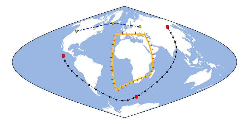
Lines can be added to a map with m.add_line().

A line is defined by a list of anchor-points and a connection-method
The coordinates of the anchor-points can be provided in any crs
Possible connection-methods are:
- connect="geod": connect points via geodesic lines (the default)
  - use n=10 to calculate 10 intermediate points between each anchor-point
  - or use del_s=1000 to calculate intermediate points (approximately) every 1000 meters
    
    check the return-values of m.add_line() to get the actual distances used in each line-segment
- connect="straight": connect points via straight lines
- connect="straight_crs": connect points with reprojected lines that are straight in a given projection
  - use n=10 to calculate 10 (equally-spaced) intermediate points between each anchor-point
Additional keyword-arguments are passed to matpltolib’s plt.plot
- This gives a lot of flexibility to style the lines!

add_line

Draw a line by connecting a set of anchor-points.

from eomaps import Maps
import matplotlib.patheffects as path_effects

m = Maps(Maps.CRS.Sinusoidal(), figsize=(8, 4))
m.add_feature.preset.ocean()

p0 = [(-100,10), (34, -56), (125, 57)]
p1 = [(-120,50), (-42, 63), (45, 57)]
p2 = [(-20,-45), (-20, 45), (45, 45), (45, -20), (-20,-45)]


m.add_line(p0, connect="geod", del_s=100000,
           lw=0.5, c="k", mark_points="rs",
           marker=".", markevery=10)

m.add_line(p1, connect="straight", c="b", ls="--",
           mark_points=dict(fc="y", ec="k", lw=.5))

m.add_line(p2, connect="straight_crs", c="r",
           n=5, lw=0.25, ms=5,
           path_effects=[
               path_effects.withStroke(linewidth=3,
                                       foreground="gold"),
               path_effects.TickedStroke(angle=90,
                                         linewidth=1,
                                         length=0.5)])

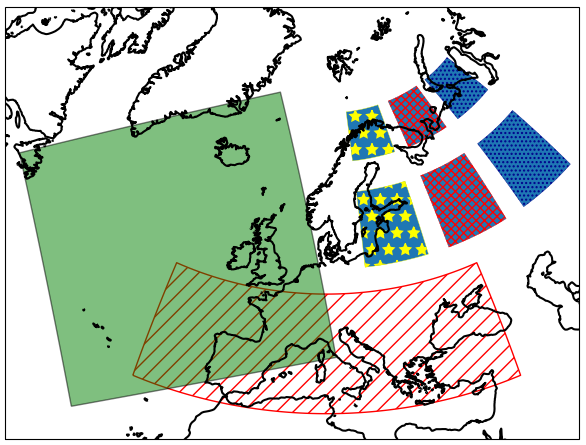
▭ Rectangular areas

To indicate rectangular areas in any given crs, simply use m.indicate_extent:

indicate_extent

Indicate a rectangular extent in a given crs on the map.

from eomaps import Maps
m = Maps(crs=3035)
m.add_feature.preset.coastline(ec="k")

# indicate a lon/lat rectangle
m.indicate_extent(-20, 35, 40, 50, hatch="//", fc="none", ec="r")

# indicate some rectangles in epsg:3035
hatches = ["*", "xxxx", "...."]
colors = ["yellow", "r", "darkblue"]
for i, h, c in zip(range(3), hatches, colors):
    pos0 = (2e6 + i*2e6, 7e6, 3.5e6 + i*2e6, 9e6)
    pos1 = (2e6 + i*2e6, 7e6 + 3e6, 3.5e6 + i*2e6, 9e6 + 3e6)

    m.indicate_extent(*pos0, crs=3857, hatch=h, lw=0.25, ec=c)
    m.indicate_extent(*pos1, crs=3857, hatch=h, lw=0.25, ec=c)

# indicate a rectangle in Equi7Grid projection
try: # (requires equi7grid package)
    m.indicate_extent(1000000, 1000000, 4800000, 4800000,
                      crs=Maps.CRS.Equi7Grid_projection("EU"),
                      fc="g", alpha=0.5, ec="k")
except:
    pass

🥦 Logos

To add a logo (or basically any image file .png, .jpeg etc.) to the map, you can use m.add_logo.

Logos can be re-positioned and re-sized with the 🏗️ Layout Editor!

To fix the relative position of the logo with respect to the map-axis, use fix_position=True

from eomaps import Maps
m = Maps()
m.add_feature.preset.coastline()
m.add_logo(position="ul", size=.15)
m.add_logo(position="ur", size=.15)
# notice that the bottom logos maintain their relative position on resize/zoom events!
# (and also that they can NOT be moved with the layout-editor)
m.add_logo(position="lr", size=.3, pad=(0.1,0.05), fix_position=True)
m.add_logo(position="ll", size=.4, fix_position=True)

add_logo

Add a small image (png, jpeg etc.) to the map whose position is dynamically updated if the plot is resized or zoomed.

🌈 Colorbars (with a histogram)

Before adding a colorbar, you must plot the data using m.plot_map().

A colorbar with a colored histogram on top can then be added to the map via m.add_colorbar.

Note

Colorbars are only visible if the layer at which the data was plotted is visible!

m = Maps(layer=0)
...
m.add_colorbar()   # this colorbar is only visible on the layer 0

m2 = m.new_layer("data")
...
m2.add_colorbar()  # this colorbar is only visible on the "data" layer

add_colorbar

Add a colorbar to the map.

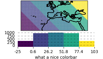
from eomaps import Maps
import numpy as np
x, y = np.mgrid[-45:45, 20:60]

m = Maps()
m.add_feature.preset.coastline()
m.set_data(data=x+y, x=x, y=y, crs=4326)
m.set_classify_specs(scheme=Maps.CLASSIFIERS.EqualInterval, k=5)
m.plot_map()
m.add_colorbar(label="what a nice colorbar", histbins="bins")

Note

You must plot a dataset first! (e.g. by calling m.plot_map())
The colorbar always represents the dataset that was used in the last call to m.plot_map().
If you need multiple colorbars, use an individual Maps object for each dataset! (e.g. via m2  = m.new_layer())

Once the colorbar has been created, the colorbar-object can be accessed via m.colorbar. It has the following useful methods defined:

`set_position`	Set the position of the colorbar (and all colorbars that share the same location)
`set_hist_size`	Set the size of the histogram (relative to the total colorbar size)
`tick_params`
`set_visible`	Set the visibility of the colorbar
`remove`	Remove the colorbar from the map.

📎 Set colorbar tick labels based on bins

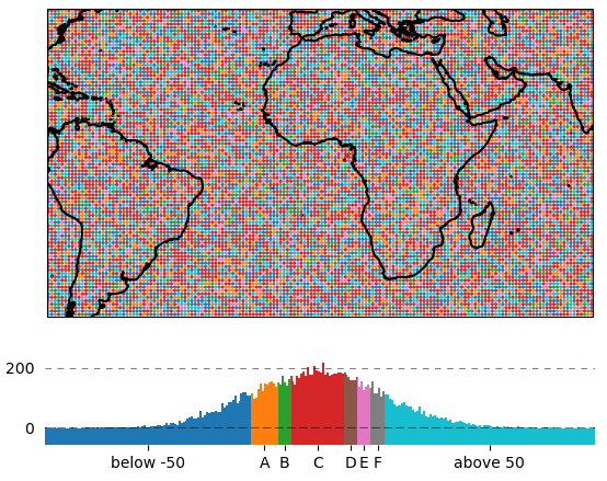
To label the colorbar with custom names for a given set of bins, use m.colorbar.set_bin_labels():

import numpy as np
from eomaps import Maps
# specify some random data
lon, lat = np.mgrid[-45:45, -45:45]
data = np.random.normal(0, 50, lon.shape)

# use a custom set of bins to classify the data
bins = np.array([-50, -30, -20, 20, 30, 40, 50])
names = np.array(["below -50", "A", "B", "C", "D", "E", "F", "above 50"])

m = Maps()
m.add_feature.preset.coastline()
m.set_data(data, lon, lat)
m.set_classify.UserDefined(bins=bins)
m.plot_map(cmap="tab10")
m.add_colorbar()

# set custom colorbar-ticks based on the bins
m.colorbar.set_bin_labels(bins, names)

set_bin_labels

Set the tick-labels of the colorbar to custom names with respect to a given set of bins.

🌠 Using the colorbar as a “dynamic shade indicator”

If you use shade_raster or shade_points as plot-shape, the colorbar can be used to indicate the distribution of the shaded pixels within the current field of view by setting dynamic_shade_indicator=True.

from eomaps import Maps
import numpy as np
x, y = np.mgrid[-45:45, 20:60]

m = Maps()
m.add_feature.preset.coastline()
m.set_data(data=x+y, x=x, y=y, crs=4326)
m.set_shape.shade_raster()
m.plot_map()
m.add_colorbar(dynamic_shade_indicator=True, histbins=20)

📏 Scalebars

A scalebar can be added to a map via s = m.add_scalebar():

add_scalebar

Add a scalebar to the map.

from eomaps import Maps
m = Maps(Maps.CRS.Sinusoidal())
m.add_feature.preset.ocean()
s = m.add_scalebar()

Note

The scalebar is a pickable object! Click on it with the LEFT mouse button to drag it around, and use the RIGHT mouse button to make it fixed again.

If the scalebar is picked (indicated by a red border), you can use the following keys for adjusting some of the ScaleBar properties:

delte: remove the scalebar from the plot
+ and -: rotate the scalebar
up/down/left/right: increase the size of the frame
alt + up/down/left/right: decrease the size of the frame

The returned ScaleBar object provides the following useful methods:

`ScaleBar.remove`	Remove the scalebar from the map
`ScaleBar.set_position`	Set the position of the colorbar
`ScaleBar.get_position`	Return the current position (and orientation) of the scalebar (e.g.
`ScaleBar.set_label_props`	Set the properties of the labels (and update the plot accordingly)
`ScaleBar.set_patch_props`	Set the properties of the frame (and update the plot accordingly)
`ScaleBar.set_scale_props`	Set the properties of the scalebar (and update the plot accordingly)
`ScaleBar.cb_offset_interval`	Get/set the interval for the text-offset when using the <alt> + <+>/<-> keyboard-shortcut to set the offset for the scalebar-labels.
`ScaleBar.cb_rotate_interval`	Get/set the interval for the rotation when using the <+> and <-> keys on the keyboard to rotate the scalebar

🧭 Compass (or North Arrow)

A compass can be added to the map via m.add_compass():

To add a North-Arrow, use m.add_compass(style="north arrow")

Note

The compass is a pickable object!

Click on it with the LEFT mouse button to drag it around!

While a compass is picked (and the LEFT mouse button is pressed), the following additional interactions are available:

press delte on the keyboard: remove the compass from the plot
rotate the mouse wheel: scale the size of the compass

add_compass

Add a "compass" or "north-arrow" to the map.

from eomaps import Maps
m = Maps(Maps.CRS.Stereographic())
m.add_feature.preset.ocean()

m.add_compass()

The compass object is dynamically updated if you pan/zoom the map, and it can be dragged around on the map with the mouse.

The returned compass object has the following useful methods assigned:

`set_patch`	Set the style of the background patch.
`set_scale`	Set the size of the compass.
`set_pickable`	Set if the compass can be picked with the mouse or not.
`set_ignore_invalid_angles`	Set how to deal with invalid rotation-angles.
`remove`	Remove the compass from the map.

🦜 Utility widgets

Some helpful utility widgets can be added to a map via m.util.<...>

Maps.util

A collection of utility tools that can be added to EOmaps plots

Layer switching

To simplify switching between layers, there are currently 2 widgets available:

m.util.layer_selector() : Add a set of clickable buttons to the map that activates the corresponding layers.
m.util.layer_slider() : Add a slider to the map that iterates through the available layers.

By default, the widgets will show all available layers (except the “all” layer) and the widget will be automatically updated whenever a new layer is created on the map.

To show only a subset of layers, provide an explicit list via: layers=[...layer names...].
To exclude certain layers from the widget, use exclude_layers=[...layer-names to exclude...]
To remove a previously created widget s from the map, simply use s.remove()

`layer_selector`	A button-widget that can be used to select the displayed plot-layer.
`layer_slider`	Get a slider-widget that can be used to switch between layers.

from eomaps import Maps
m = Maps(layer="coastline")
m.add_feature.preset.coastline()

m2 = m.new_layer(layer="ocean")
m2.add_feature.preset.ocean()

s = m.util.layer_selector()

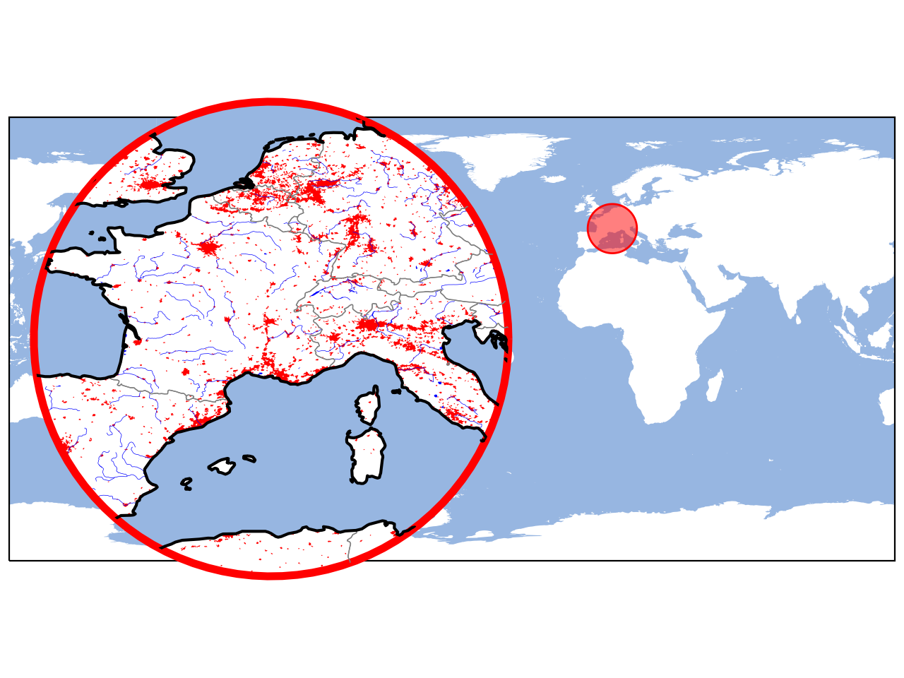
🔬 Inset-maps - zoom-in on interesting areas

Inset maps that show zoomed-in regions can be created with m.new_inset_map().

m = Maps()                                  # the "parent" Maps-object (e.g. the "big" map)
m.add_feature.preset.coastline()
m2 = m.new_inset_map(xy=(5, 5), radius=10)  # a new Maps-object that represents the inset-map
m2.add_feature.preset.ocean()               # it can be used just like any other Maps-objects!

An inset-map is defined by it’s center-position and a radius
The used boundary-shape can be one of:
- “ellipses” (e.g. projected ellipses with a radius defined in a given crs)
- “rectangles” (e.g. projected rectangles with a radius defined in a given crs)
- “geod_circles” (e.g. geodesic circles with a radius defined in meters)

For convenience, inset-map objects have the following special methods defined:

m.set_inset_position(): Set the size and (center) position of the inset-map relative to the figure size.
m.indicate_inset_extent(): Indicate the extent of the inset-map on arbitrary Maps-objects.

Checkout the associated example on how to use inset-maps: 🔬 Inset-maps - get a zoomed-in view on selected areas

Make sure to checkout the 🏗️ Layout Editor which can be used to quickly re-position (and re-size) inset-maps with the mouse!

m = Maps(Maps.CRS.PlateCarree(central_longitude=-60))
m.add_feature.preset.ocean()
m2 = m.new_inset_map(xy=(5, 45), radius=10,
                     plot_position=(.3, .5), plot_size=.7,
                     boundary=dict(ec="r", lw=4),
                     indicate_extent=dict(fc=(1,0,0,.5),
                                          ec="r", lw=1)
                     )
m2.add_feature.preset.coastline()
m2.add_feature.preset.countries()
m2.add_feature.preset.ocean()

m2.add_feature.cultural_10m.urban_areas(fc="r")
m2.add_feature.physical_10m.rivers_europe(ec="b", lw=0.25,
                                          fc="none")
m2.add_feature.physical_10m.lakes_europe(fc="b")

new_inset_map

Create a new (empty) inset-map that shows a zoomed-in view on a given extent.

✏️ Draw Shapes on the map

Starting with EOmaps v5.0 it is possible to draw simple shapes on the map using m.draw.

The shapes can be saved to disk as geo-coded shapefiles using m.draw.save_shapes(filepath).

(Saving shapes requires the geopandas module!)
To remove the most recently drawn shape use m.draw.remove_last_shape().

m = Maps()
m.add_feature.preset.coastline()
m.draw.polygon()

Note

Drawing capabilities are fully integrated in the 🧰 Companion Widget. In most cases it is much more convenient to draw shapes with the widget instead of executing the commands in a console!

In case you still stick to using the commands for drawing shape, it is important to know that the calls for drawing shapes are non-blocking and starting a new draw will silently cancel active draws!

`ShapeDrawer.new_drawer`	Initialize a new ShapeDrawer.
`ShapeDrawer.rectangle`	Draw a rectangle.
`ShapeDrawer.circle`	Draw a circle.
`ShapeDrawer.polygon`	Draw arbitarary polygons
`ShapeDrawer.save_shapes`
`ShapeDrawer.remove_last_shape`	Remove the most recently plotted polygon from the map.

🏗️ Layout Editor

EOmaps provides a Layout Editor that can be used to quickly re-arrange the positions of all axes of a figure. You can use it to simply drag the axes the mouse to the desired locations and change their size with the scroll-wheel.

Keyboard shortcuts are assigned as follows:

press ALT + L: enter the Layout Editor mode

press ALT + L again or escape to exit the Layout Editor

Pick and re-arrange the axes as you like with the mouse.

To pick multiple axes, hold down shift!
Resize picked axes with the scroll-wheel (or with the + and - keys)

For “colorbars” there are some special options:

Hold down h or v to change horizontal/vertical size
Hold down control to change ratio between colorbar and histogram

Press keys 1-9 to set the grid-spacing for the “snap-to-grid” functionality

Press 0 to deactivate “snap-to-grid”

Save and restore layouts

Once a layout (e.g. the desired position of the axes within a figure) has been arranged, the layout can be saved and re-applied with:

🌟 m.get_layout(): get the current layout (or dump the layout as a json-file)
🌟 m.apply_layout(): apply a given layout (or load and apply the layout from a json-file)

It is also possible to enter the Layout Editor and save the layout automatically on exit with:

🌟 m.edit_layout(filepath=...): enter LayoutEditor and save layout as a json-file on exit

Note

A layout can only be restored if the number (and order) of the axes remains the same! In other words:

you always need to save a new layout-file after adding additional axes (or colorbars!) to a map

`get_layout`	Get the positions of all axes within the current plot.
`apply_layout`	Set the positions of all axes within the current plot based on a previously defined layout.
`edit_layout`	Activate the "layout-editor" to quickly re-arrange the positions of subplots.

📦 Reading data (NetCDF, GeoTIFF, CSV…)

EOmaps provides some basic capabilities to read and plot directly from commonly used file-types.

By default, the Maps.from_file and m.new_layer_from_file functions try to plot the data with shade_raster (if it fails it will fallback to shade_points and finally to ellipses).

Note

At the moment, the readers are intended as a “shortcut” to read well-structured datasets! If they fail, simply read the data manually and then set the data as usual via m.set_data(...).

Under the hood, EOmaps uses the following libraries to read data:

GeoTIFF (rioxarray + xarray.open_dataset)
NetCDF (xarray.open_dataset)
CSV (pandas.read_csv)

Read relevant data from a file

m.read_file.<filetype>(...) can be used to read all relevant data (e.g. values, coordinates & crs) from a file.

m = Maps()
data = m.read_file.NetCDF(
    "the filepath",
    parameter="adsf",
    coords=("longitude", "latitude"),
    data_crs=4326,
    isel=dict(time=123)
    )
m.set_data(**data)
...
m.plot_map()

`read_file.GeoTIFF`	Read all relevant information necessary to add a GeoTIFF to the map.
`read_file.NetCDF`	Read all relevant information necessary to add a NetCDF to the map.
`read_file.CSV`	Read all relevant information necessary to add a CSV-file to the map.

Initialize Maps-objects from a file

Maps.from_file.<filetype>(...) can be used to directly initialize a Maps object from a file. (This is particularly useful if you have a well-defined file-structure that you need to access regularly)

m = Maps.from_file.GeoTIFF(
    "the filepath",
    classify_specs=dict(Maps.CLASSFIERS.Quantiles, k=10),
    cmap="RdBu"
    )
m.add_colorbar()
m.cb.pick.attach.annotate()

`from_file.GeoTIFF`	Convenience function to initialize a new Maps-object from a GeoTIFF file.
`from_file.NetCDF`	Convenience function to initialize a new Maps-object from a NetCDF file.
`from_file.CSV`	Convenience function to initialize a new Maps-object from a CSV file.

Add new layers to existing Maps-objects from a file

Similar to Maps.from_file, a new layer based on a file can be added to an existing Maps object via Maps.new_layer_from_file.<filetype>(...).

m = Maps8()
m.add_feature.preset.coastline()

m2 = m.new_layer_from_file(
    "the filepath",
    parameter="adsf",
    coords=("longitude", "latitude"),
    data_crs=4326,
    isel=dict(time=123),
    classify_specs=dict(Maps.CLASSFIERS.Quantiles, k=10),
    cmap="RdBu"
    )

`new_layer_from_file.GeoTIFF`	Convenience function to initialize a new Maps-object from a GeoTIFF file.
`new_layer_from_file.NetCDF`	Convenience function to initialize a new Maps-object from a NetCDF file.
`new_layer_from_file.CSV`	Convenience function to initialize a new Maps-object from a CSV file.

🔸 Miscellaneous

some additional functions and properties that might come in handy:

`Maps.on_layer_activation`	Attach a callback that is executed if the associated layer is activated.
`Maps.set_extent_to_location`	Set the map-extent based on a given location query.
`Maps.get_crs`	Get the pyproj CRS instance of a given crs specification
`Maps.indicate_masked_points`	Add circles to the map that indicate masked points.
`Maps.show`	Make the layer of this Maps-object visible.
`Maps.show_layer`	Display the selected layer on the map.
`Maps.BM`	The Blit-Manager used to dynamically update the plots
`Maps.join_limits`	Join the x- and y- limits of the axes (e.g.
`Maps.snapshot`	Print a static image of the current figure to the active IPython display.