🌱 Basics

Getting started 

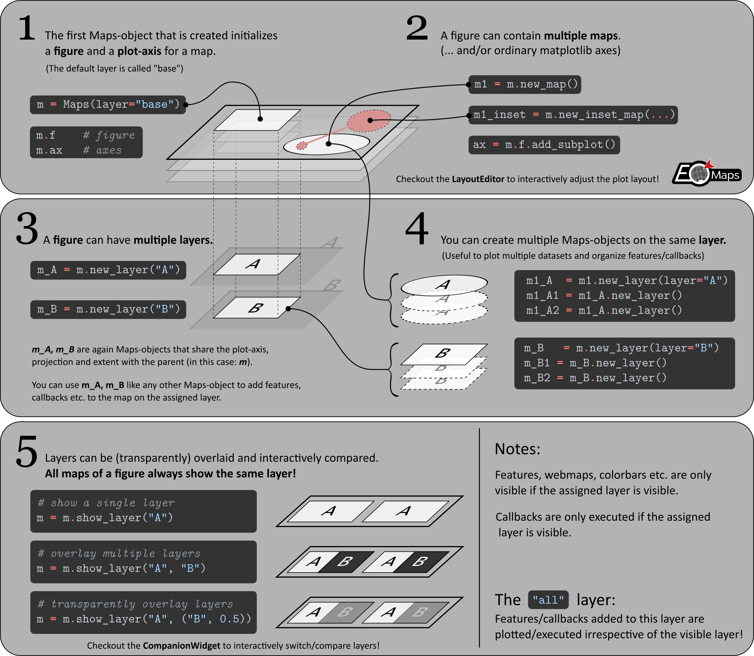
EOmaps is all about Maps objects.

The first Maps object that is created will initialize a matplotlib.Figure and a cartopy.GeoAxes for a map.

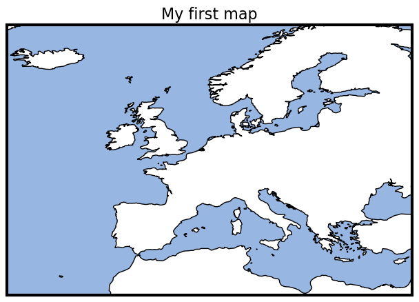
from eomaps import Maps
m = Maps(                        # Create a Maps-object
    crs=4326,                    #     Use lon/lat (epsg=4326) projection
    layer="base",                #     Assign the layer-name "base"
    figsize=(6, 5))              #     Set the figure-size to 6x5

m.set_extent((-25, 35, 30, 70))  # Set the extent of the map
m.set_frame(linewidth=3)         # Set the linewidth of the frame

m.add_feature.preset.coastline() # Add coastlines
m.add_feature.preset.ocean()     # Add ocean-coloring
m.add_title("My first map",      # Add a title
            fontsize=16)         #     With a fontsize of 16pt

crs represents the projection used for plotting
layer represents the name of the layer associated with the Maps-object (see Layer management).
all additional keyword arguments are forwarded to the creation of the matplotlib-figure (e.g.: figsize, frameon, edgecolor etc).

`Maps`	The base-class for generating plots with EOmaps.
`Maps.CRS`	The crs module defines Coordinate Reference Systems and the transformations between them.
`Maps.set_extent`	Set the extent (x0, x1, y0, y1) of the map in the given coordinate system.
`Maps.add_title`	Convenience function to add a title to the map.

Layer management 

A Maps object represents one (or more) of the following things on the assigned layer:

a collection of features, callbacks,..
a single dataset (and associated callbacks)

You can create as many layers as you need! The following image explains how it works in general:

🗗 Combine & compare multiple layers

All maps of a figure always show the same visible layer.

The visible layer can be a single layer-name, or a combination of multiple layer-names in order to to transparently combine/overlay multiple layers.

`Maps.new_layer`	Create a new Maps-object that shares the same plot-axes.
`Maps.all`	Get a Maps-object on the "all" layer.
`Maps.show`	Show the map (only required for non-interactive matplotlib backends).
`Maps.show_layer`	Show a single layer or (transparently) overlay multiple selected layers.
`Maps.fetch_layers`	Fetch (and cache) the layers of a map.

Image export (jpeg, png, svg, etc.)

Once the map is ready, an image of the map can be saved at any time by using Maps.savefig()

from eomaps import Maps
m = Maps()
m.add_feature.preset.ocean()
m.savefig("snapshot1.png", dpi=200, transparent=True)

To adjust the margins of the subplots, use m.subplots_adjust(), or have a look at the 🏗️ Layout Editor!

from eomaps import Maps
m = Maps()
m.subplots_adjust(left=0.1, right=0.9, bottom=0.05, top=0.95)

`Maps.savefig`	Save the current figure.
`Maps.subplots_adjust`	Update the subplot parameters of the grid.
`Maps.set_clipboard_kwargs`	Set GLOBAL savefig parameters for all Maps objects on export to the clipboard.

Multiple Maps (and/or plots) in one figure 

It is possible to combine multiple EOmaps maps and/or ordinary matpltolib plots in one figure.

The figure used by a Maps object is set via the f argument, e.g.: m = Maps(f=...). If no figure is provided, a new figure is created whenever you initialize a Maps object. The figure-instance of an existing Maps object is accessible via m.f

To add a map to an existing figure, use m2 = m.new_map() (requires EOmaps >= v6.1) or pass the figure-instance on initialization of a new Maps object.
To add a ordinary matplotlib plot to a figure containing an eomaps-map, use m.f.add_subplot() or m.f.add_axes().

The initial position of the axes used by a Maps object is set via the ax argument, e.g.: m = Maps(ax=...) or m2 = m.new_map(ax=...)

The syntax for positioning axes is similar to matplotlibs f.add_subplot() or f.add_axes()
The axis-instance of an existing Maps object is accessible via m.ax
…for more information, checkout the matplotlib tutorial: Customizing Figure Layouts

Note

Make sure to have a look at the 🏗️ Layout Editor on how to re-position and re-scale axes to arbitrary positions!

`Maps`	The base-class for generating plots with EOmaps.
`Maps.new_map`	Create a new map that shares the figure with this Maps-object.

In the following, the most commonly used cases are introduced:

Grid positioning

To position the map in a (virtual) grid, one of the following options are possible:

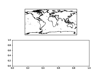
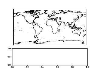
Three integers (nrows, ncols, index) (or 2 integers and a tuple).
- The map will take the index position on a grid with nrows rows and ncols columns.
- index starts at 1 in the upper left corner and increases to the right.
- index can also be a two-tuple specifying the (first, last) indices (1-based, and including last) of the map, e.g., Maps(ax=(3, 1, (1, 2))) makes a map that spans the upper 2/3 of the figure.

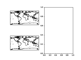
from eomaps import Maps
# ----- initialize a figure with an EOmaps map
# position = item 1 of a 2x1 grid
m = Maps(ax=(2, 1, 1))
# ----- add a normal matplotlib axes
# position = item 2 of a 2x1 grid
ax = m.f.add_subplot(2, 1, 2)

from eomaps import Maps
# ----- initialize a figure with an EOmaps map
# position = item 1 of a 2x2 grid
m = Maps(ax=(2, 2, 1))
# ----- add another Map to the same figure
# position = item 3 of a 2x2 grid
m2 = m.new_map(ax=(2, 2, 3))
# ----- add a normal matplotlib axes
# position = second item of a 1x2 grid
ax = m.f.add_subplot(1, 2, 2)

from eomaps import Maps
# ----- initialize a figure with an EOmaps map
# position = item 1 of a 2x2 grid
m = Maps(ax=(2, 2, 1))
# ----- add another Map to the same figure
# position = item 3 of a 2x2 grid
m2 = m.new_map(ax=(2, 2, 3))
# ----- add a normal matplotlib axes
# position = second item of a 1x2 grid
ax = m.f.add_subplot(1, 2, 2)

A 3-digit integer.
- The digits are interpreted as if given separately as three single-digit integers, i.e. Maps(ax=235) is the same as Maps(ax=(2, 3, 5)).
- Note that this can only be used if there are no more than 9 subplots.

from eomaps import Maps
# ----- initialize a figure with an EOmaps map
m = Maps(ax=211)
# ----- add a normal matplotlib axes
ax = m.f.add_subplot(212)

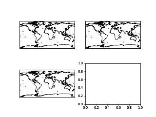
from eomaps import Maps
# ----- initialize a figure with an EOmaps map
m = Maps(ax=221)
# ----- add 2 more Maps to the same figure
m2 = m.new_map(ax=222)
m3 = m.new_map(ax=223)
# ----- add a normal matplotlib axes
ax = m.f.add_subplot(224)

A matplotlib GridSpec

from matplotlib.gridspec import GridSpec
from eomaps import Maps

gs = GridSpec(2, 2)
m = Maps(ax=gs[0,0])
m2 = m.new_map(ax=gs[0,1])
ax = m.f.add_subplot(gs[1,:])

Absolute positioning

To set the absolute position of the map, provide a list of 4 floats representing (left, bottom, width, height).

The absolute position of the map expressed in relative figure coordinates (e.g. ranging from 0 to 1)

Note

Since the effective size of the Map is dependent on the current zoom-region, the position always represents the maximal area that can be occupied by the map!

Also, using m.f.tight_layout() will not work with axes added in this way.

from eomaps import Maps
# ----- initialize a figure with an EOmaps map
m = Maps(ax=(.07, 0.53, .6, .3))
# ----- add a normal matplotlib axes
ax = m.f.add_axes((.35, .15, .6, .2))

Using already existing figures / axes

It is also possible to insert an EOmaps map into an existing figure or reuse an existing axes.

To put a map on an existing figure, provide the figure-instance via m = Maps(f= <the figure instance>)

To use an existing axes, provide the axes-instance via m = Maps(ax= <the axes instance>)

NOTE: The axes MUST be a cartopy-GeoAxes!

import matplotlib.pyplot as plt
import cartopy
from eomaps import Maps

f = plt.figure(figsize=(10, 7))
ax = f.add_subplot(projection=cartopy.crs.Mollweide())

m = Maps(f=f, ax=ax)

Dynamic updates of plots in the same figure

As soon as a Maps-object is attached to a figure, EOmaps will handle re-drawing of the figure! Therefore dynamically updated artists must be added to the “blit-manager” (m.BM) to ensure that they are correctly updated.

use m.BM.add_artist(artist, layer=...) if the artist should be re-drawn on any event in the figure

use m.BM.add_bg_artist(artist, layer=...) if the artist should only be re-drawn if the extent of the map changes

Note

In most cases it is sufficient to simply add the whole axes-object as artist via m.BM.add_artist(...).

This ensures that all artists of the axes are updated as well!

Here’s an example to show how it works:

from eomaps import Maps

# Initialize a new figure with an EOmaps map
m = Maps(ax=223)
m.ax.set_title("click me!")
m.add_feature.preset.coastline()
m.cb.click.attach.mark(radius=20, fc="none", ec="r", lw=2)

# Add another map to the figure
m2 = m.new_map(ax=224, crs=Maps.CRS.Mollweide())
m2.add_feature.preset.coastline()
m2.add_feature.preset.ocean()
m2.cb.click.attach.mark(radius=20, fc="none", ec="r", lw=2, n=200)

# Add a "normal" matplotlib plot to the figure
ax = m.f.add_subplot(211)
# Since we want to dynamically update the data on the axis, it must be
# added to the BlitManager to ensure that the artists are properly updated.
# (EOmaps handles interactive re-drawing of the figure)
m.BM.add_artist(ax, layer=m.layer)

# plot some static data on the axis
ax.plot([10, 20, 30, 40, 50], [10, 20, 30, 40, 50])

# define a callback that plots markers on the axis if you click on the map
def cb(pos, **kwargs):
    ax.plot(*pos, marker="o")

m.cb.click.attach(cb)        # attach the callback to the first map
m.cb.click.share_events(m2)  # share click events between the 2 maps

MapsGrid objects

MapsGrid objects can be used to create (and manage) multiple maps in one figure.

Note

While MapsGrid objects provide some convenience, starting with EOmaps v6.x, the preferred way of combining multiple maps and/or matplotlib axes in a figure is by using one of the options presented in the previous sections!

A MapsGrid creates a grid of Maps objects (and/or ordinary matpltolib axes), and provides convenience-functions to perform actions on all maps of the figure.

from eomaps import MapsGrid
mg = MapsGrid(r=2, c=2, crs=4326)
# you can then access the individual Maps-objects via:
mg.m_0_0.add_feature.preset.ocean()
mg.m_0_1.add_feature.preset.land()
mg.m_1_0.add_feature.preset.urban_areas()
mg.m_1_1.add_feature.preset.rivers_lake_centerlines()

m_0_0_ocean = mg.m_0_0.new_layer("ocean")
m_0_0_ocean.add_feature.preset.ocean()

# functions executed on MapsGrid objects will be executed on all Maps-objects:
mg.add_feature.preset.coastline()
mg.add_compass()

# to perform more complex actions on all Maps-objects, simply loop over the MapsGrid object
for m in mg:
    m.add_gridlines(10, c="lightblue")

# set the margins of the plot-grid
mg.subplots_adjust(left=0.1, right=0.9, bottom=0.05, top=0.95, hspace=0.1, wspace=0.05)

Make sure to checkout the 🏗️ Layout Editor which greatly simplifies the arrangement of multiple axes within a figure!

Custom grids and mixed axes

Fully customized grid-definitions can be specified by providing m_inits and/or ax_inits dictionaries of the following structure:

The keys of the dictionary are used to identify the objects
The values of the dictionary are used to identify the position of the associated axes
The position can be either an integer N, a tuple of integers or slices (row, col)
Axes that span over multiple rows or columns, can be specified via slice(start, stop)

dict(
    name1 = N  # position the axis at the Nth grid cell (counting firs)
    name2 = (row, col), # position the axis at the (row, col) grid-cell
    name3 = (row, slice(col_start, col_end)) # span the axis over multiple columns
    name4 = (slice(row_start, row_end), col) # span the axis over multiple rows
    )

m_inits is used to initialize Maps objects
ax_inits is used to initialize ordinary matplotlib axes

The individual Maps objects and matpltolib-Axes are then accessible via:

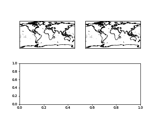
from eomaps import MapsGrid
mg = MapsGrid(2, 3,
            m_inits=dict(ocean=(0, 0), land=(0, 2)),
            ax_inits=dict(someplot=(1, slice(0, 3)))
            )
# Maps object with the name "left"
mg.m_ocean.add_feature.preset.ocean()
# the Maps object with the name "right"
mg.m_land.add_feature.preset.land()

# the ordinary matplotlib-axis with the name "someplot"
mg.ax_someplot.plot([1,2,3], marker="o")
mg.subplots_adjust(left=0.1, right=0.9, bottom=0.2, top=0.9)

❗ NOTE: if m_inits and/or ax_inits are provided, ONLY the explicitly defined objects are initialized!

The initialization of the axes is based on matplotlib’s GridSpec functionality. All additional keyword-arguments (width_ratios, height_ratios, etc.) are passed to the initialization of the GridSpec object.
To specify unique crs for each Maps object, provide a dictionary of crs specifications.

from eomaps import MapsGrid
# initialize a grid with 2 Maps objects and 1 ordinary matplotlib axes
mg = MapsGrid(2, 2,
            m_inits=dict(top_row=(0, slice(0, 2)),
                        bottom_left=(1, 0)),
            crs=dict(top_row=4326,
                    bottom_left=3857),
            ax_inits=dict(bottom_right=(1, 1)),
            width_ratios=(1, 2),
            height_ratios=(2, 1))

# a map extending over the entire top-row of the grid (in epsg=4326)
mg.m_top_row.add_feature.preset.coastline()

# a map in the bottom left corner of the grid (in epsg=3857)
mg.m_bottom_left.add_feature.preset.ocean()

# an ordinary matplotlib axes in the bottom right corner of the grid
mg.ax_bottom_right.plot([1, 2, 3], marker="o")
mg.subplots_adjust(left=0.1, right=0.9, bottom=0.1, top=0.9)

`MapsGrid`	Initialize a grid of Maps objects
`MapsGrid.join_limits`	Join axis limits between all Maps objects of the grid (only possible if all maps share the same crs!)
`MapsGrid.share_click_events`	Share click events between all Maps objects of the grid
`MapsGrid.share_pick_events`	Share pick events between all Maps objects of the grid
`MapsGrid.set_data`	This will execute the corresponding action on ALL Maps objects of the MapsGrid!
`MapsGrid.set_classify_specs`	This will execute the corresponding action on ALL Maps objects of the MapsGrid!
`MapsGrid.add_wms`	A collection of open-access WebMap services that can be added to the maps.
`MapsGrid.add_feature`	Interface to features provided by NaturalEarth.
`MapsGrid.add_annotation`	This will execute the corresponding action on ALL Maps objects of the MapsGrid!
`MapsGrid.add_marker`	This will execute the corresponding action on ALL Maps objects of the MapsGrid!
`MapsGrid.add_gdf`	This will execute the corresponding action on ALL Maps objects of the MapsGrid!

Naming conventions and autocompletion 

The goal of EOmaps is to provide a comprehensive, yet easy-to-use interface.

To avoid having to remember a lot of names, a concise naming-convention is applied so that autocompletion can quickly narrow-down the search to relevant functions and properties.

Once a few basics keywords have been remembered, finding the right functions and properties should be quick and easy.

Note

EOmaps works best in conjunction with “dynamic autocompletion”, e.g. by using an interactive console where you instantiate a Maps object first and then access dynamically updated properties and docstrings on the object.

To clarify:

First, execute m = Maps() in an interactive console
then (inside the console, not inside the editor!) use autocompletion on m. to get autocompletion for dynamically updated attributes.

For example the following accessors only work properly after the Maps object has been initialized

Maps.add_wms browse available WebMap services
Maps.set_classify browse available classification schemes

The following list provides an overview of the naming-conventions used within EOmaps:

Add features to a map - “m.add_”

All functions that add features to a map start with add_, e.g.:

Maps.add_feature, Maps.add_wms, Maps.add_annotation(), Maps.add_marker(), Maps.add_gdf(), …

WebMap services (e.g. Maps.add_wms) are fetched dynamically from the respective APIs. Therefore the structure can vary from one WMS to another. The used convention is the following:

You can navigate into the structure of the API by using “dot-access” continuously
once you reach a level that provides layers that can be added to the map, the .add_layer. directive will be visible
any <LAYER> returned by .add_layer.<LAYER> can be added to the map by simply calling it, e.g.:
- m.add_wms.OpenStreetMap.add_layer.default()
- m.add_wms.OpenStreetMap.OSM_mundialis.add_layer.OSM_WMS()

Set data specifications - “m.set_”

All functions that set properties of the associated dataset start with set_, e.g.:

Maps.set_data(), Maps.set_classify, Maps.set_shape, …

Create new Maps-objects - “m.new_”

Actions that result in a new Maps objects start with new_.

Maps.new_layer(), Maps.new_inset_map(), …

Callbacks - “m.cb.”

Everything related to callbacks is grouped under the cb accessor.

use m.cb.<METHOD>.attach.<CALLBACK>() to attach pre-defined callbacks
- <METHOD> hereby can be one of click, pick or keypress (but there’s no need to remember since autocompletion will do the job!).
use m.cb.<METHOD>.attach(custom_cb) to attach a custom callback

🌱 Basics

Getting started

Layer management

🗗 Combine & compare multiple layers

Image export (jpeg, png, svg, etc.)

Multiple Maps (and/or plots) in one figure

Grid positioning

Absolute positioning

Using already existing figures / axes

Dynamic updates of plots in the same figure

MapsGrid objects

Custom grids and mixed axes

Naming conventions and autocompletion

Add features to a map - “m.add_”

Set data specifications - “m.set_”

Create new Maps-objects - “m.new_”

Callbacks - “m.cb.”

Getting started 

Layer management 

Multiple Maps (and/or plots) in one figure 

Naming conventions and autocompletion 